Screen 28-day concrete strength before committing to laboratory trials
This surrogate model estimates 28-day compressive strength from seven constituent quantities. It helps concrete technologists compare candidate mixtures and focus physical testing on the most promising, feasible formulations.
Compressive-strength testing is essential, but each result arrives only after batching, curing and destructive laboratory testing. A data-driven surrogate can provide rapid estimates for screening and scenario analysis, while qualified mix design, trial batches and standards-based testing remain the basis for production and structural decisions.
1. Industrial challenge
This is an approximation problem: the model maps seven constituent quantities to the continuous target compressive_strength, measured in MPa after 28 days.
Potential users include ready-mix and precast producers, concrete technologists, materials laboratories, civil and structural engineers, quality teams and low-carbon construction specialists.
2. Data set
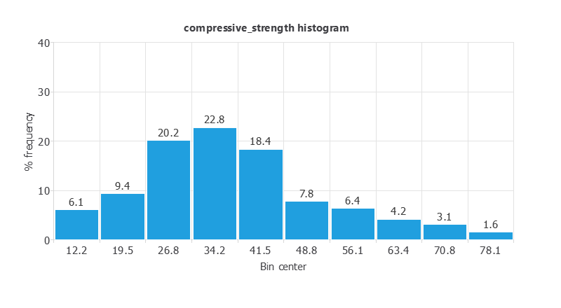
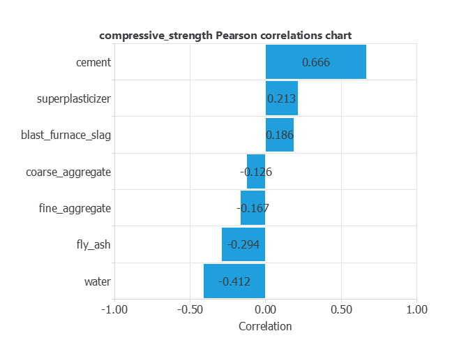
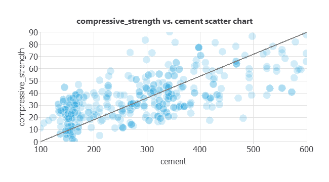
The source UCI Concrete Compressive Strength dataset contains 1,030 laboratory results with age as an input. This example uses all 425 records tested at 28 days, so age is fixed and omitted from the local file. The semicolon-delimited CSV contains seven numerical inputs, one numerical target and no missing values.
| CSV variable | Engineering meaning | Role | Unit | Observed range |
|---|---|---|---|---|
cement | Cement | Input | kg/m³ | 102 to 540 |
blast_furnace_slag | Blast-furnace slag | Input | kg/m³ | 0 to 359.4 |
fly_ash | Fly ash | Input | kg/m³ | 0 to 200.1 |
water | Water | Input | kg/m³ | 121.8 to 247 |
superplasticizer | Superplasticizer | Input | kg/m³ | 0 to 32.2 |
coarse_aggregate | Coarse aggregate | Input | kg/m³ | 801 to 1145 |
fine_aggregate | Fine aggregate | Input | kg/m³ | 594 to 992.6 |
compressive_strength | 28-day compressive strength | Target | MPa | 8.54 to 81.75 |
The configured random split assigns 255 rows to training, 85 to selection and 85 to testing.
3. Neural network
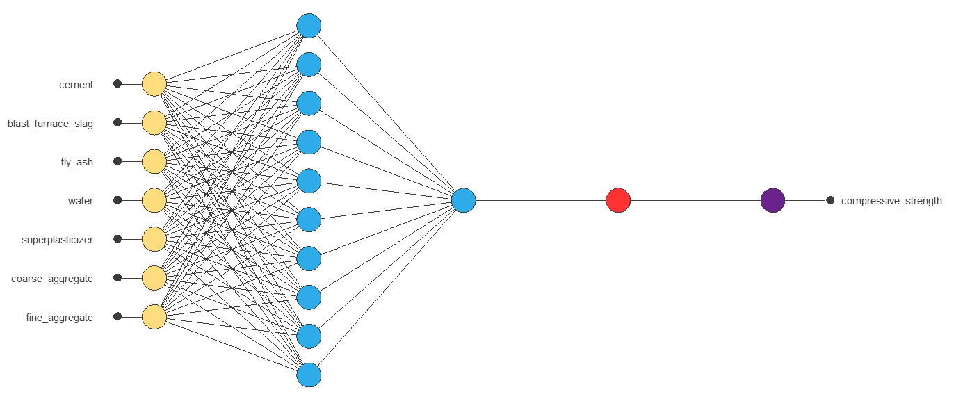
The initial model standardizes seven inputs using mean and standard deviation, evaluates three tanh hidden neurons and returns one linear strength estimate before unscaling to MPa. The initial 7–3–1 architecture contains 28 trainable parameters.
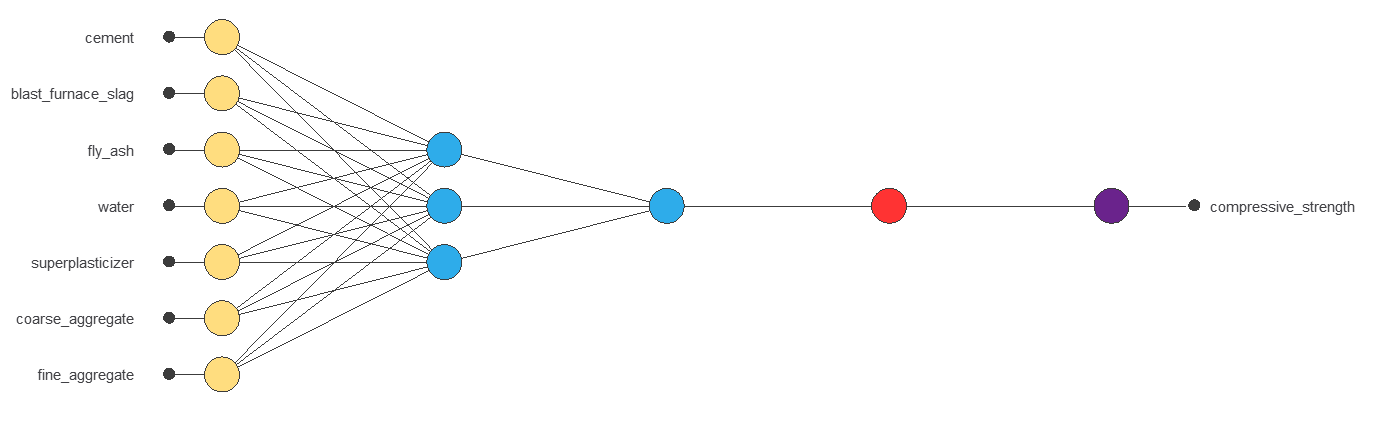
The initial network provides a compact starting point. Model selection subsequently changes the hidden-layer size; the final testing and deployment model is shown in section 5.
4. Training strategy
The initial network minimizes normalized squared error with L2 regularization weight 0.01 using the quasi-Newton method. Optimization stops after 78 epochs because the minimum loss decrease criterion is reached. The recorded training and selection errors are 0.098 NSE and 0.049 NSE.
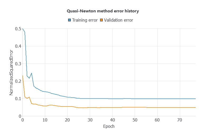
Normalized squared error is useful during optimization, but MPa-based metrics are used later so engineering users can interpret the practical size of prediction errors.
5. Model selection
The growing-neurons task compares hidden-layer sizes from 1 to 10, using three trials per size. The smallest recorded selection error, 0.0429 NSE, occurs at 10 neurons; the corresponding training error is 0.083 NSE.
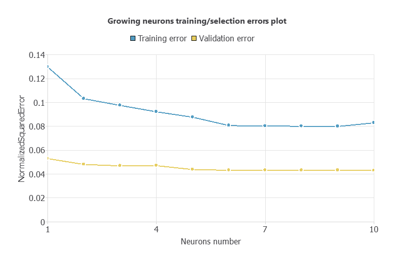
Because the best result occurs at the configured maximum, 10 neurons is the best tested size rather than proof of a global optimum. The final 7–10–1 network contains 91 trainable parameters and is the model used for testing, optimization and Python export.
6. Testing analysis
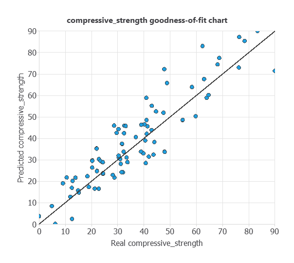
The exported final model was recalculated on the 85 rows marked as testing. R² is the squared correlation reported by the Neural Designer goodness-of-fit analysis; MAE and RMSE express errors directly in MPa.
| Testing rows | R² | MAE | RMSE | Bias | 95th-percentile absolute error | Maximum absolute error |
|---|---|---|---|---|---|---|
| 85 | 0.8214 | 4.88 MPa | 6.06 MPa | +0.68 MPa | 10.70 MPa | 19.34 MPa |
A training-mean baseline has an RMSE of 14.22 MPa, so the neural model materially improves on a constant prediction. Nevertheless, only 56.5% of testing rows fall within ±5 MPa, and the largest error is operationally significant. This supports screening use, not automatic acceptance.
7. Model deployment
A practical workflow starts with a physically feasible formulation and ends with laboratory confirmation. The model can screen or rank candidates, but engineering constraints must be applied before inference and predictions must not become production specifications without validation.
Optimization case 1: reduce cement for a 45 MPa requirement
Operational question: what is the lowest-cement candidate that provides a modelled safety margin above a required 28-day strength of 45 MPa?
The executed task minimizes cement, keeps the other constituents inside defined operating intervals and requires a predicted strength of at least 55 MPa. The additional 10 MPa is an illustrative screening margin informed by the model error; it is not a certified characteristic-strength calculation or prediction interval.
| Variable | Condition | Lower bound | Upper bound | Optimized value | Unit |
|---|---|---|---|---|---|
| Cement | Minimize | — | — | 126.513 | kg/m³ |
| Blast-furnace slag | Between | 50 | 220 | 219.710 | kg/m³ |
| Fly ash | Between | 0 | 150 | 139.026 | kg/m³ |
| Water | Between | 160 | 195 | 172.402 | kg/m³ |
| Superplasticizer | Between | 0 | 15 | 14.277 | kg/m³ |
| Coarse aggregate | Between | 850 | 1,075 | 1,060.860 | kg/m³ |
| Fine aggregate | Between | 650 | 875 | 869.364 | kg/m³ |
| Compressive strength | ≥ | 55 | — | 55.000 | MPa |
Result and engineering interpretation
| Check | Candidate | Observed data domain | Assessment |
|---|---|---|---|
| Total binder | 485.249 kg/m³ | 200.0–640.0 kg/m³ | Inside observed interval |
| Water-to-binder ratio | 0.355 | 0.235–0.900 | Inside observed interval |
| Total constituent mass | 2,602.152 kg/m³ | 2,194.6–2,551.0 kg/m³ | 51.2 kg/m³ above observed maximum |
The optimizer reduces cement by moving slag close to its upper bound and using substantial fly ash, superplasticizer and aggregate quantities. The model reproduces the requested 55 MPa threshold, but the constituent total is approximately 2.0% above the largest formulation in the dataset. The candidate therefore demonstrates a credible low-cement objective, yet it still requires a mass-balance or yield constraint and laboratory validation before it can be considered a feasible mix.
Optimization case 2: maximize strength with cement capped at 300 kg/m³
Operational question: what is the highest 28-day strength predicted inside the declared constituent limits when cement cannot exceed 300 kg/m³?
This scenario maximizes the model output while bounding cement and every other constituent. It represents a producer seeking higher strength without moving to a high-cement formulation.
| Variable | Condition | Lower bound | Upper bound | Optimized value | Unit |
|---|---|---|---|---|---|
| Cement | Between | 200 | 300 | 299.998 | kg/m³ |
| Blast-furnace slag | Between | 0 | 220 | 220.000 | kg/m³ |
| Fly ash | Between | 0 | 150 | 149.499 | kg/m³ |
| Water | Between | 155 | 190 | 178.930 | kg/m³ |
| Superplasticizer | Between | 0 | 15 | 13.390 | kg/m³ |
| Coarse aggregate | Between | 850 | 1,075 | 1,075.000 | kg/m³ |
| Fine aggregate | Between | 650 | 875 | 874.735 | kg/m³ |
| Compressive strength | Maximize | — | — | 80.156 | MPa |
Result and engineering interpretation
| Check | Candidate | Observed data domain | Assessment |
|---|---|---|---|
| Total binder | 669.497 kg/m³ | 200.0–640.0 kg/m³ | 29.5 kg/m³ above observed maximum |
| Water-to-binder ratio | 0.267 | 0.235–0.900 | Inside observed interval |
| Total constituent mass | 2,811.552 kg/m³ | 2,194.6–2,551.0 kg/m³ | 260.6 kg/m³ above observed maximum |
The solution reaches 80.156 MPa by driving cement, slag, fly ash and both aggregates to, or very close to, their upper bounds. This is a typical boundary-seeking optimizer response. Although the individual values satisfy the declared limits, binder content and total mass lie outside every mixture represented in the data. The result is best interpreted as a diagnostic upper-bound scenario: it shows why a real maximum-strength optimization also needs total-binder, yield, workability, cost and durability constraints.
Comparison of the two executed cases
| Scenario | Primary objective | Cement | Predicted strength | Total mass | Current status |
|---|---|---|---|---|---|
| Low-cement target-strength case | Minimize cement with predicted strength ≥55 MPa | 126.513 kg/m³ | 55.000 MPa | 2,602.152 kg/m³ | Promising objective; revise mass balance |
| Cement-capped maximum-strength case | Maximize strength with cement ≤300 kg/m³ | 299.998 kg/m³ | 80.156 MPa | 2,811.552 kg/m³ | Boundary result; reformulate constraints |
Cement sensitivity at a reference formulation
At 265 kg/m³ cement, 86 kg/m³ slag, 62 kg/m³ fly ash, 183 kg/m³ water, 7 kg/m³ superplasticizer, 956 kg/m³ coarse aggregate and 764 kg/m³ fine aggregate, the model predicts 37.47 MPa. The directional plot varies cement while holding the other quantities fixed.
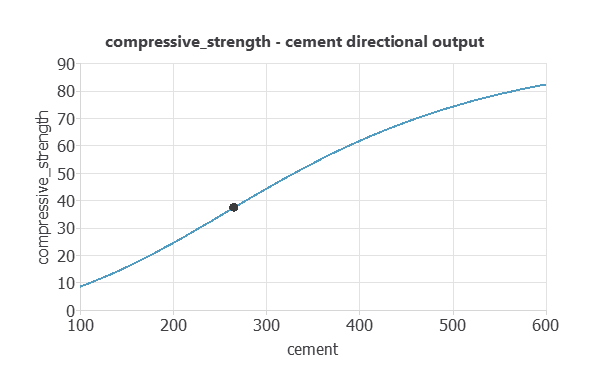
Interpret the curve only across the observed cement interval of 102–540 kg/m³. The portion beyond 540 kg/m³ is model extrapolation and should not support a design decision.
Try the 28-day strength model
Enter one mixture or load a verified example. The browser evaluates the exact scaling, weights and output transformation from the exported Python model.
Screening model — not a certified mix design, conformity assessment or structural acceptance method.
Download and reproduce
Video walkthrough
The original tutorial remains available as a step-by-step Neural Designer walkthrough. Numerical results on this page reflect the newly exported project.
8. Scope and limitations
- The model represents 28-day strength only. It cannot estimate early-age or long-term strength because age is fixed and absent from the inputs.
- The data comes from a public laboratory collection and does not establish transfer to a specific plant, cement source, aggregate grading, admixture product, curing regime or test procedure.
- Random row splitting and duplicated formulations can produce a more optimistic test than validation by unseen formulation family, production batch or chronological campaign.
- The target is compressive strength only; workability, slump, density, durability, heat, shrinkage, cost and embodied carbon are not modelled.
- Inputs are constituent masses, but the model does not enforce volume balance, total yield, water-to-binder limits, aggregate proportions or material compatibility.
- The observed range of each variable does not define a valid multidimensional mixture domain. Joint feasibility must be checked separately.
- Production deployment requires local data, grouped or time-aware validation, drift monitoring, uncertainty limits and periodic recalibration.
- Predictions support screening and experimentation; qualified personnel and standards-based testing remain responsible for mix approval and structural acceptance.
References
- Yeh, I.-C. Concrete Compressive Strength Dataset, UCI Machine Learning Repository, DOI: 10.24432/C5PK67.
- Yeh, I.-C. Modeling of strength of high-performance concrete using artificial neural networks, Cement and Concrete Research 28(12), 1797–1808 (1998).
- Neural Designer testing analysis: goodness-of-fit and regression metrics.
- Neural Designer model deployment: directional outputs, response optimization and model export.