1. Application type
This is an approximation project since the variable to be predicted is continuous (residuary resistance).
The primary goal here is to model the residuary resistance of a yacht as a function of its geometry and speed.
2. Data set
The first step is to prepare the data set, which is the source of information for the approximation problem. It contains the following three concepts:
- Data source.
- Variables.
- Instances.
The file yacht_hydrodynamics.csv contains the data for this example. Here the number of instances (rows) is 308, and the number of variables (columns) is 7.
The data set contains the following variables:
- center_of_buoyancy: Longitudinal position of the center of buoyancy, dimensionless. Used as an input.
- prismatic_coefficient: Prismatic coefficient, dimensionless. Used as an input.
- length_displacement: Length-displacement ratio, dimensionless. Used as an input.
- beam_draught_ratio: Beam-draught ratio, dimensionless. Used as an input.
- length_beam_ratio: Length-beam ratio, dimensionless. Used as an input.
- froude_number: Froude number, dimensionless. Used as an input.
- resistance: Residuary resistance per unit weight of displacement, dimensionless. Used as the target.
Note that the variables used (input, target, or unused) must be selected carefully. Any application must have one or more inputs and one or more targets.
Finally, the instances are divided into training, validation, and testing subsets. Here, the instances are split randomly with ratios 0.6, 0.2, and 0.2. More specifically, 186 instances are used for training, 61 for validation, and 61 for testing.
Once we edit the data set page, we will run a few related tasks. With that, we check that the provided information is of good quality.
We can calculate the data distributions and draw a histogram for each variable to see how they are distributed. The following figure shows the histogram for the resistance data, which is the only target.
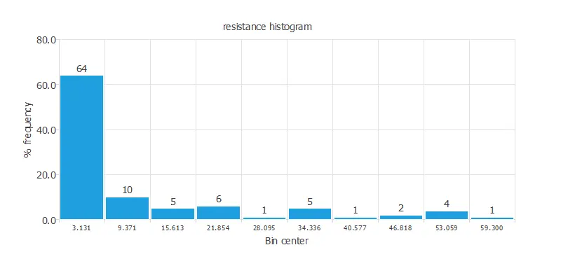
As we can see, most of the data is concentrated at low resistance values.
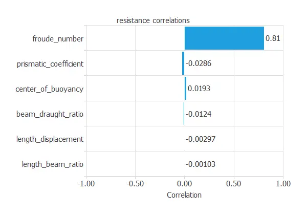
The following figure shows the input variables’ correlations with the target variable.
3. Neural network
The second step is to set the neural network stuff. For approximation, project types typically consist of:
- Scaling layer.
- Perceptron layers.
- Unscaling layer.
- Bounding layer.
The scaling layer section contains the statistics on the inputs calculated from the data file and the method for scaling the input variables. Here, we have set the minimum and maximum methods. Nevertheless, the mean and standard deviation method would produce very similar results.
In this problem, we will use a hidden sigmoid layer and a linear output layer of perceptrons, the default approximation.
It must have six inputs and one output neuron. While the problem constrains inputs and output neurons, the number of neurons in the hidden layer is a design variable. Here, we use six neurons in the hidden layer, which yields 49 parameters. Finally, all the biases and synaptic weights in the neural network are initialized randomly.
The unscaling layer contains the statistics on the outputs calculated from the data file and the method for unscaling the output variables. Here, we will also utilize the minimum and maximum methods.
We can represent the neural network for this example in the following diagram:
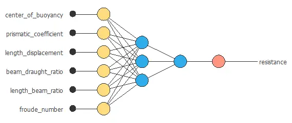
All the biases and synaptic weights in the neural network parameterize the function above, totaling 49 parameters.
4. Training strategy
The next step is selecting an appropriate training strategy to define what the neural network will learn. A general training strategy for approximation comprises two components:
- A loss index.
- An optimization algorithm.
The loss index chosen for this problem is the normalized squared error between the neural network outputs and the data set’s targets. On the other hand, no regularization will be used for this application.
The selected optimization algorithm is the quasi-Newton method.
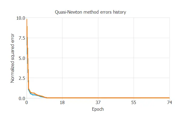
The most crucial training result is the final selection error. Indeed, this is a measure of the generalization capabilities of the neural network. Here, the final selection error is selection error = 0.007 NSE.
5. Model selection
Model selection algorithms are used to improve the generalization performance of the neural network.
As the selection error achieved so far is minimal (0.007 NSE), these algorithms are unnecessary here.
6. Testing analysis
The next step is to perform a testing analysis to measure the generalization performance of the neural network. Here, we compare the values provided by this technique to the observed values. Since testing has no settings, there is no testing analysis page in Neural Designer.
A common testing technique for the neural network model is to perform a linear regression analysis Using an independent testing set between the predicted and corresponding experimental residuary resistance values. The following figure illustrates a graphical output provided by this testing analysis.
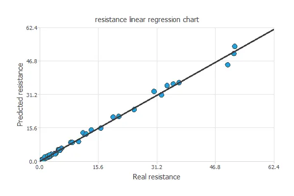
The solid line indicates the best linear fit. The dashed line with R2 = 1 would show a perfect fit. We can see from the information above that the neural network predicts the entire range of residuary resistance data. Indeed R2 value is very close to 1.
The neural network is now ready to estimate the residuary resistance of sailing yachts with satisfactory quality over the same range of data.
7. Model deployment
The neural network is now ready to predict resistances for geometries and velocities it has never seen. For that, we can use some neural network tasks.
The objective of the Response Optimization algorithm is to exploit the mathematical model to look for optimal operating conditions. Indeed, the predictive model allows us to simulate different operating scenarios and adjust the control variables to improve efficiency.
An example is to minimize a yacht residuary resistance while maintaining the center of buoyancy between two desired values.
The next table resumes the conditions for this problem.
| Variable name | Condition | ||
|---|---|---|---|
| Center of buoyancy | Between | -3 | -2 |
| Prismatic coefficient | None | ||
| Length displacement | None | ||
| Beam draught ratio | None | ||
| Length beam ratio | None | ||
| Froude number | None | ||
| Resistance | Minimize |
The next list shows the optimum values for previous conditions.
- center_of_buoyancy: -2.59598.
- prismatic_coefficient: 0.555675.
- length_displacement: 4.59281.
- beam_draught_ratio: 4.44246.
- length_beam_ratio: 3.25657.
- froude_number: 0.191938
- resistance: 0.0111761.
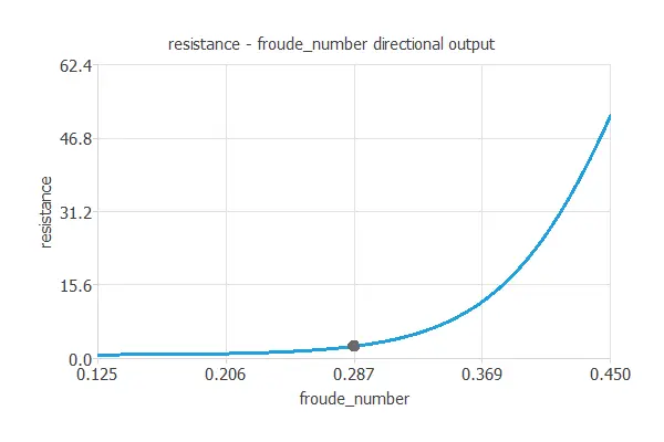
Directional outputs plot the resistance as a function of a given input for all the other fixed to given values. The next figures show the directional inputs dialog and the corresponding directional output. Here, we want to see how the resistance varies with the center of buoyancy for the following variables fixed:
- Prismatic coefficient: 0.6
- Length displacement: 4.34
- Beam daughter ratio: 4.23
- Length beam ratio: 2.73
- Froude number: 0.45
The explicit expression for the residuary resistance model obtained by the neural network is listed below.
scaled_center_of_buoyancy = 2*(center_of_buoyancy+5)/(0+5)-1;
scaled_prismatic_coefficient = (prismatic_coefficient-0.564136)/0.02329;
scaled_length_displacement = 2*(length_displacement-4.34)/(5.14-4.34)-1;
scaled_beam_draught_ratio = (beam_draught_ratio-3.93682)/0.548193;
scaled_length_beam_ratio = 2*(length_beam_ratio-2.73)/(3.64-2.73)-1;
scaled_froude_number = 2*(froude_number-0.125)/(0.45-0.125)-1;
y_1_1 = tanh (-2.15185+ (scaled_center_of_buoyancy*0.0336499)+ (scaled_prismatic_coefficient*0.0022637)+ (scaled_length_displacement*0.203965)+ (scaled_beam_draught_ratio*-0.126716)+ (scaled_length_beam_ratio*-0.239965)+ (scaled_froude_number*1.89048));
scaled_resistance =  (1.17499+ (y_1_1*2.15355));
resistance = (0.5*(scaled_resistance+1.0)*(62.42-0.01)+0.01);
According to these predictions, the above expression could be exported elsewhere to design yachts.
References
- UCI Machine Learning Repository. Yacht Hydrodynamics Data Set.
- Ortigosa, I., Lopez, R., & Garcia, J. (2007). A neural networks approach to residuary resistance of sailing yachts prediction. In Proceedings of the international conference on marine engineering MARINE (Vol. 2007, p. 250).