Learning

Build a digital twin of an electric motor using machine learning

Predict critical motor temperatures without instrumenting the rotor

This data-driven thermal digital twin estimates four internal temperatures from eight routinely available operating signals. It can support overheating prevention, cooling studies and safer operating limits for permanent-magnet synchronous motors.

8operating inputs

4predicted temperatures

0.923average testing R²

175steady-state operating points

Try the digital twin Download the data

Temperature is one of the main operating constraints in an electric motor. Excess heat accelerates winding-insulation ageing and can permanently damage rotor magnets, but rotor temperature is difficult to measure in a deployed machine.

This example shows how a neural network can act as a steady-state thermal soft sensor: speed, torque, voltages, currents and cooling conditions are converted into estimates of stator-yoke, stator-tooth, winding and permanent-magnet temperature.

The model was built with Neural Designer. The downloadable data and Python deployment package make the workflow reproducible.

Industrial challenge
Data set
Neural network
Training strategy
Model selection
Testing analysis
Model deployment
Limitations
References

1. Industrial challenge

This is an approximation project. The model maps an electric motor operating point to the temperatures reached inside the machine.

Protect critical componentsEstimate winding and permanent-magnet temperature before thermal limits are exceeded.

Evaluate operating scenariosStudy how cooling and electrical conditions influence internal temperatures without risking physical hardware.

Deploy a thermal soft sensorUse signals already available from a controller, test bench, PLC or supervisory system.

Potential users include motor and drivetrain engineers, reliability teams, test-bench operators, production leaders and Industry 4.0 teams:

Plant operationsReliability & maintenanceMotor engineeringTest benchesDigital transformation

Scope of this example. This is a data-driven, steady-state thermal digital twin. In production it would become the predictive core of a real-time monitoring workflow, connected to live signals, alarms and model-performance monitoring.

2. Data set

The first step is to prepare the data set, which is the source of information for the approximation problem. It is composed of:

Data source.
Variables.
Instances.

Data source

The file electric_motor.csv contains the data for this example. The original recordings are taken several times per second, so consecutive rows are almost identical, and many of them belong to changing driving cycles. To describe the motor properly, we keep one representative value for each stable operating condition: a fixed speed and torque, once the temperatures have settled. This gives a clean data set of 175 instances with 13 columns.

Variables

This problem has the following variables:

session_id, identifier of the measurement session. It is only used to keep track of the experiments, not as an input or a target.
ambient_temperature, ambient temperature measured by a thermal sensor located close to the stator.
coolant_temperature, coolant temperature. The motor is water-cooled. Measurement is taken at the outflow.
speed, motor speed.
torque, torque induced by the current.
voltage_d, voltage d-component.
voltage_q, voltage q-component.
current_d, current d-component.
current_q, current q-component.
yoke_temperature, stator yoke temperature measured with a thermal sensor.
tooth_temperature, stator tooth temperature measured with a thermal sensor.
winding_temperature, stator winding temperature measured with a thermal sensor.
magnet_temperature, rotor permanent-magnet temperature.

The variables ‘ambient_temperature’, ‘coolant_temperature’, ‘speed’, ‘torque’, ‘voltage_d’, ‘voltage_q’, ‘current_d’, and ‘current_q’ are the inputs. They describe the operating point of the motor (the cooling conditions and the electrical excitation). On the contrary, ‘yoke_temperature’, ‘tooth_temperature’, ‘winding_temperature’, and ‘magnet_temperature’ are the targets of this study. Our main goal is to describe the behavior of the electric motor to prevent overheating, so these output variables are the temperatures of the engine’s internal parts: three in the stator and one in the rotor.

Instances

They are divided randomly into training, selection, and testing subsets, containing 60%, 20%, and 20% of the instances, respectively. More specifically, 105 samples are used here for training, 35 for validation, and 35 for testing.

Variables distribution

Once we establish the data set information, we perform analytics to check the data quality. For instance, we can calculate the data distribution. The next figure depicts the histogram for one of the target variables.

In this diagram, we can see a normal distribution of the stator tooth temperature, one of the parts of the stator. This output depends on many input variables at the same time, so its values spread across the whole range instead of concentrating on a single value.

Inputs-targets correlations

The next figure depicts inputs-targets correlations. This might help us see the different inputs’ influence on the motor temperature. As this machine learning study has several target variables, we show the correlation diagram for the stator winding and for the rotor magnet.

winding_temperature Pearson correlations chart

magnet_temperature Pearson correlations chart

The stator temperatures depend mostly on the coolant and the currents, as expected in a water-cooled machine. The rotor magnet, however, is related to a wider mix of inputs, which is a first sign that it will be the most difficult temperature to predict.

Scatter charts

We can also plot a scatter chart with the stator winding temperature versus the ambient temperature.

winding_temperature vs. ambient_temperature scatter chart

Logically, the higher the ambient temperature, the higher the stator winding temperature.

3. Neural network

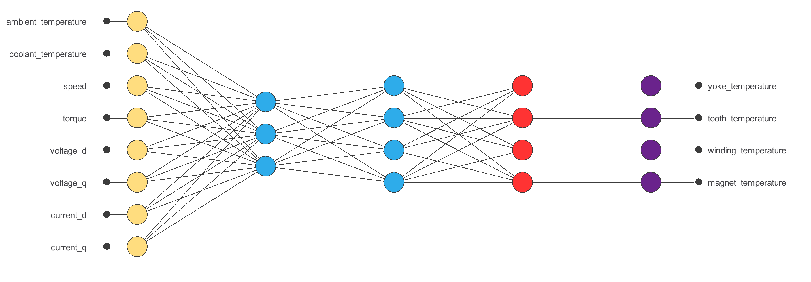
The initial model uses the same eight operating signals and four temperature targets as the rest of the study. A scaling layer standardizes the inputs, a dense layer with four tanh neurons learns nonlinear thermal relationships, and the output layer returns the four temperatures in degrees Celsius.

This compact 8–4–4 architecture provides the baseline for training before the hidden-layer size is refined during model selection.

Initial neural network with eight operating inputs, four hidden neurons and four motor temperature outputs

4. Training strategy

The next step is selecting an appropriate training strategy to define what the neural network will learn. A general training strategy is composed of two concepts:

A loss index.
An optimization algorithm.

The loss index chosen is the normalized squared error with L2 regularization. This loss index is the default in approximation applications. The optimization algorithm chosen is the quasi-Newton method. This optimization algorithm is the default for medium-sized applications like this one. Once the strategy has been set, we can train the neural network. The following chart shows how the training (blue) and selection (orange) errors decrease with the training epoch during the training process.

The most critical training result is the final selection error. Indeed, this is a measure of the generalization capabilities of the neural network. After 89 epochs, the final training error is 0.0333 NSE and the final selection error is 0.0166 NSE.

5. Model selection

The objective of model selection is to find the network architecture with the best generalization properties. We want to improve the final selection error obtained before (0.0166 NSE). The best selection error is achieved using a model whose complexity is the most appropriate to produce a good data fit. Order selection algorithms are responsible for finding the optimal number of perceptrons in the neural network. The final training error continuously decreases with the number of neurons. However, the final selection error takes a minimum value at some point. Here, the optimal number of neurons is 7, corresponding to a selection error of 0.0133 NSE. The following figure shows the optimal network architecture for this application.

Selected neural network with eight operating inputs, seven hidden neurons and four motor temperature outputs

6. Testing analysis

The objective of the testing analysis is to validate the generalization performance of the trained neural network. The testing compares the values provided by this technique to the observed values. A standard testing technique in approximation problems is to perform a linear regression analysis between the predicted and the real values using an independent testing set. The 35 held-out testing samples are evaluated with the coefficient of determination (R²) and with absolute errors expressed in degrees Celsius. MAE describes the typical absolute deviation, while RMSE gives more weight to larger errors.

Predicted temperature	R²	MAE	RMSE
Stator yoke	0.976	3.14 °C	3.65 °C
Stator tooth	0.951	4.58 °C	5.38 °C
Stator winding	0.934	6.85 °C	7.78 °C
Rotor magnet	0.833	6.51 °C	8.44 °C
Average	0.923	5.27 °C	6.31 °C

The stator yoke gives the strongest result (R² = 0.976; MAE = 3.14 °C). The rotor magnet is more difficult to estimate because it is thermally isolated and its temperature depends on a complex combination of operating conditions. Its testing MAE is 6.51 °C. This is also a high-value prediction because direct rotor instrumentation is difficult in deployed equipment. The following figures illustrate the graphical output provided by this testing analysis, one per target. The closer the points are to the grey line, the better the prediction.

Validation note. The reported results use the random 60/20/20 split configured in this example. Because several operating points can belong to the same measurement session, an industrial validation should also reserve complete sessions or driving cycles for testing. This gives a more conservative estimate of performance on unseen experiments.

Stator tooth predicted versus measured temperature — **Stator tooth**
R² 0.951 · MAE 4.58 °C

Stator winding predicted versus measured temperature — **Stator winding**
R² 0.934 · MAE 6.85 °C

Rotor magnet predicted versus measured temperature — **Rotor magnet**
R² 0.833 · MAE 6.51 °C

Stator yoke predicted versus measured temperature — **Stator yoke**
R² 0.976 · MAE 3.14 °C

7. Model deployment

In an industrial application, the neural network acts as a thermal soft sensor. Signals already available from a controller, test bench, PLC or SCADA system are transformed into estimates of temperatures that are expensive or impractical to measure continuously.

PLC, controller or test bench

8 operating signals

Thermal digital twin

Temperatures, alarms and decisions

Try the thermal digital twin

Enter an operating point within the training ranges. The calculation runs locally in your browser using the same weights and preprocessing as the exported Python model.

Stator yoke—

Stator tooth—

Stator winding—

Rotor magnet—

Demonstration model — not a certified thermal protection system.

From prediction to response optimization

A directional-output chart is useful for sensitivity analysis, but an operational study should focus on a decision such as maintaining required speed and torque while reducing thermal stress. A suitable response-optimization problem would minimize the highest predicted winding or magnet temperature, subject to feasible cooling and motor-control constraints.

ObjectiveMinimize max(winding temperature, magnet temperature).

Operating requirementsKeep the requested speed and torque and respect voltage, current and cooling limits.

Engineering constraintOnly evaluate combinations that are physically achievable by the motor-control strategy.

The most useful next visualization would be a speed–torque operating map coloured by predicted magnet or winding temperature, with safe, caution and thermal-limit regions. A second useful chart would compare temperature against coolant temperature at a fixed production duty point.

Important. The calculator demonstrates model inference inside the data ranges. It is not a certified protection function, and optimization recommendations must be validated against motor physics and plant safety requirements.

Download and integrate

The deployment package contains electric_motor.py, including input scaling, trained neural-network weights, output unscaling and temperature bounds.

Download Python model (ZIP)Download dataset (CSV)

8. Scope and limitations

The data represents one permanent-magnet synchronous motor on a test bench and 175 selected steady-state operating points.
The model should not be extrapolated beyond the input ranges shown in the calculator.
Dynamic warm-up, transient loads and long-term thermal ageing are not modelled explicitly.
A different motor, cooling circuit or control strategy requires new validation and may require retraining.
Production deployment should monitor missing signals, sensor quality, model drift and prediction error.
The model supports engineering decisions; it does not replace certified motor-protection systems.

References

Kaggle Machine Learning Repository. Electric Motor Temperature Data Set.