Customer churn is a big problem for telecommunications companies.
Indeed, their annual churn rates are usually higher than 10%.
Therefore, they must develop strategies to keep as many clients as possible.
This example uses machine learning to predict which customers will leave the company, take measures to prevent it, and implement strategies accordingly.
Contents
1. Application type
This is a classification project since the variable to be predicted is binary (churn or loyal customer).
The goal is to model churn probability conditioned on the customer features.
2. Data set
The data file telecommunications_churn.csv contains a total of 19 features for 3333 customers.
Each row corresponds to a client of a telecommunications company for whom information has been collected about the type of plan they have contracted, the minutes they have talked, or the charge they pay every month.
Variables
The data set includes the following variables:
Customer Profile
- account_length: Number of months the customer has been with the company.
- customer_service_calls: Number of calls made by the customer to the service center.
Service Plans
- voice_mail_plan: Whether the customer has subscribed to a voicemail plan (yes/no).
- voice_mail_messages: Number of voicemail messages recorded.
- international_plan: Whether the customer has subscribed to an international plan (yes/no).
Usage (Minutes and Calls)
- day_mins: Total minutes of calls made during the day.
- day_calls: Total number of calls made during the day.
- evening_mins: Total minutes of calls made in the evening.
- evening_calls: Total number of calls made in the evening.
- night_mins: Total minutes of calls made at night.
- night_calls: Total number of calls made at night.
- international_mins: Total minutes of international calls.
- international_calls: Total number of international calls.
Billing (Charges)
- day_charge: Total charges for calls made during the day.
- evening_charge: Total charges for calls made in the evening.
- night_charge: Total charges for calls made at night.
- international_charge: Total charges for international calls.
- total_charge: Overall charges (sum of day, evening, night, and international charges).
Target Variable
churn: Indicates whether the customer has left the company (1) or stayed (0).
Variables distribution
The first step of this analysis is to check the distributions of the variables. The following figure shows a pie chart of churn and loyal customers.
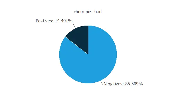
As we can see, the annual churn rate in this company is almost 15%. Also, we observe that the dataset is unbalanced.
Inputs-targets correlations
The inputs-targets correlations might indicate to us what factors are most influential for the churn of customers.
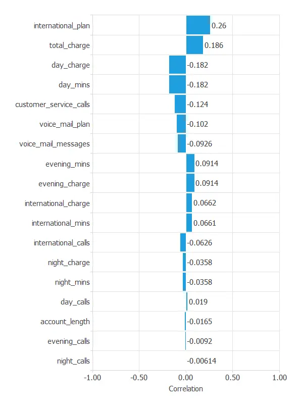
Here, the most correlated variable with churn is international_plan. A positive correlation here means that a high ratio of customers with an international plan leaves the company.
2. Neural network
The second step is to choose a neural network to represent the classification function. For classification problems, it is composed of:
Scaling layer
For the scaling layer, the mean and standard deviation scaling method is set.
Perceptron layers
We set 2 perceptron layers, one hidden layer with 3 neurons as a first guess and one output layer with 1 neuron, both layers having the logistic activation function.
Probabilistic layer
Finally, we will implement the continuous probabilistic method for the probabilistic layer.
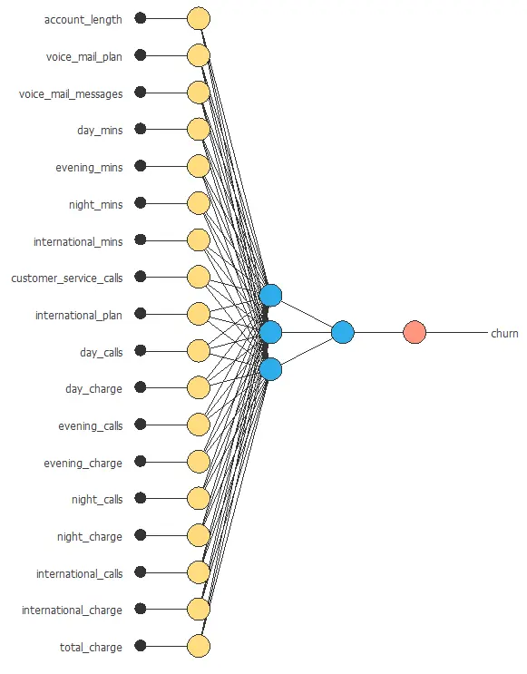
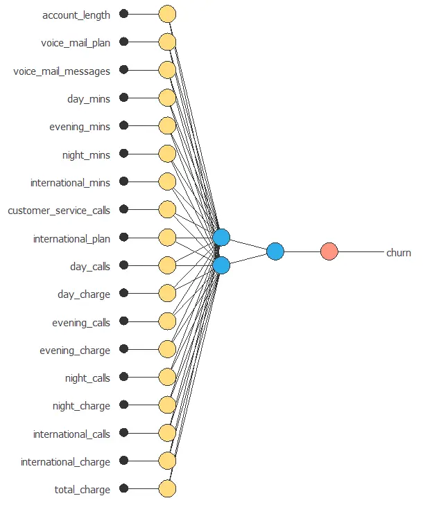
Network architecture
The architecture shown below consists of 18 scaling neurons (yellow), five neurons in the first layer (blue), and one probabilistic neuron (red).
4. Training strategy
The next step is to select an appropriate training strategy that defines what the neural network will learn. A general training strategy is composed of two concepts:
- A loss index.
- An optimization algorithm.
Loss index
As we saw before, the data set is unbalanced. In that way, we set the weighted squared error.
Training process
The following chart shows how the loss decreases during the training process with the iterations of the Quasi-Newton method.
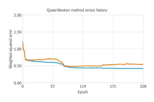
As we can see, the final training and selection errors are training error = 0.384 WSE and selection error = 0.455 WSE, respectively.
5. Model selection
The objective of model selection is to find the network architecture with the best generalization properties, which minimizes the error on the selected instances of the data set.
We aim to develop a neural network with a selection error of less than 0.455 WSE, which is the value we have achieved so far.
Order selection algorithms train several network architectures with a different number of neurons and select that with the most minor selection error.
The incremental order method starts with a few neurons and increases the complexity at each iteration.
The following chart shows the training error (blue) and the selection error (orange) as a function of the number of neurons.
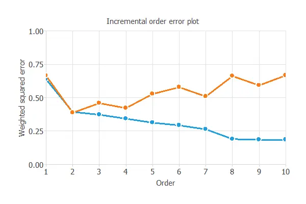
As we can see, the optimal number of perceptrons in the first layer is 2, and the optimum error on the selected instances is 0.455 WSE.
6. Testing analysis
The testing analysis aims to evaluate the performance of the trained model on new data that have not been used for training or selection.
For that, we use the testing instances.
ROC curve
The ROC curve measures the discrimination capacity of the classifier between positive and negative instances.
The following chart shows the ROC curve of our problem.
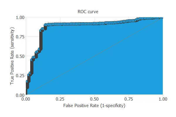
The proximity of the curve to the upper left corner means that the model has an excellent capacity to discriminate between the two classes.
The most important parameter from the ROC curve is the area under the curve (AUC). This value is 0.5 for a random classifier and 1 for a perfect classifier.
For this example, we have AUC = 0.896, indicating that the model performs well in predicting our customers’ churn.
Confusion matrix
The following figure shows the confusion matrix.
| Predicted positive | Predicted negative | |
|---|---|---|
| Real positive | 316 (15.8%) | 96 (4.8%) |
| Real negative | 325 (16.3%) | 1263 (63.1%) |
The binary classification tests are calculated from the values of the confusion matrix.
- Classification accuracy: 91.2% (ratio of correctly classified samples).
- Error rate: 8.8% (ratio of misclassified samples).
- Sensitivity: 76.9% (percentage of actual positives classified as positive).
- Specificity: 93.9% (percentage of actual negatives classified as negative).
These binary classification tests show that the model can predict most instances correctly.
7. Model deployment
In the model deployment phase, the neural network can predict outputs for inputs it has never seen.
Neural network outputs
We can calculate the neural network outputs for a given set of inputs:
- account_length: 101.065.
- voice_mail_plan: 1.
- voice_mail_messages: 8.09901.
- day_mins: 179.775.
- evening_mins: 200.98.
- night_mins: 200.871.
- international_mins: 10.2373.
- customer_service_calls: 1.56286.
- international_plan: 0.
- day_calls: 100.436.
- day_charge: 30.5623.
- evening_calls: 100.114.
- evening_charge: 17.0835.
- night_calls: 100.108.
- night_charge: 9.03933.
- international_calls: 4.47945.
- international_charge: 2.76457.
- total_charge: 59.4498.
The predicted churn for these inputs is the following:
- churn: 0.047.