
This post examines three key methods for handling outliers in machine learning.
Outliers are data points that are distant from the rest.
They may be due to variability in the measurement or may indicate experimental errors.
If possible, outliers should be excluded from the dataset.
However, detecting anomalous instances might be difficult and is not always possible.
The data science and machine learning platform Neural Designer encompasses all these methods, enabling their practical application. You can download a free trial here.
Introduction
Machine learning algorithms are susceptible to the statistics and distribution of the input variables.
Data outliers can spoil and mislead the training process.
That results in longer training times, less accurate models, and poor results.
In this post, we introduce three different methods of dealing with outliers:
- Univariate method: This method identifies data points with extreme values on a single variable.
- Multivariate method: Here, we look for unusual combinations of all the variables.
- Minkowski error: This method reduces the contribution of potential outliers in the training process.
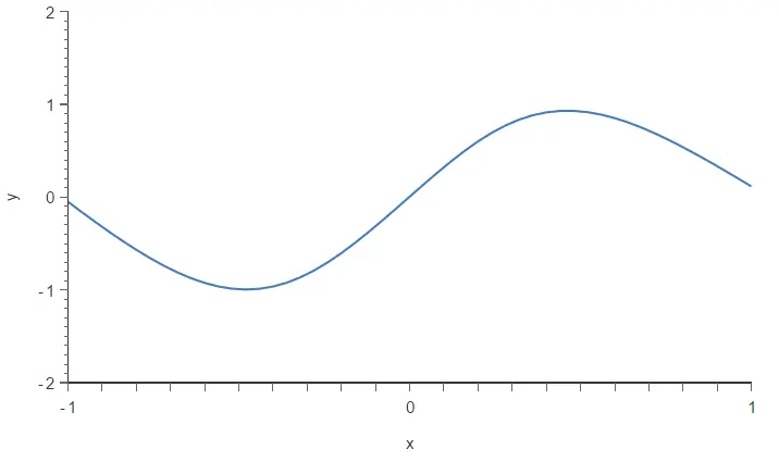
To illustrate those methods, we generate a data set from the following function
$$y = sin{(pi x)}$$
Then, we replace two (y) values for those far from our function. The following chart depicts this data set.
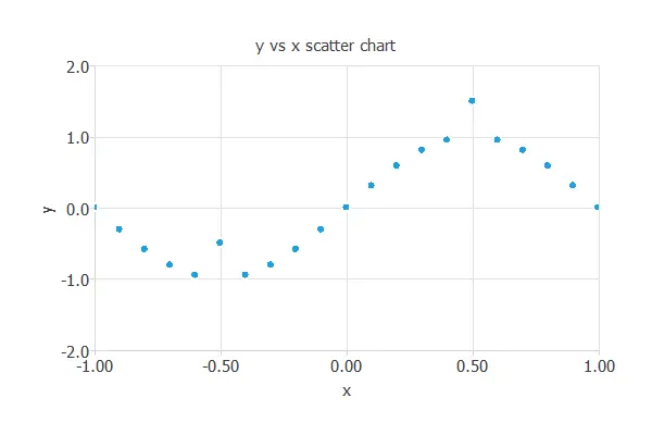
The points A=(-0.5,-1.5) and B=(0.5,0.5) are outliers.
Point (A) is outside the range defined by the (y) data, while Point (B) is inside that range. As we will see, that makes them different, and we will need different methods to detect and treat them.
1. Univariate method
One of the simplest methods for detecting outliers is using box plots.
A box plot is a graphical display that describes the data distribution. Box plots use the median and the lower and upper quartiles.
Tukey’s method defines an outlier as a value of a variable that falls far from the central point, the median.
The cleaning parameter is the maximum distance to the median that will be allowed. The test becomes less sensitive to outliers if the cleaning parameter is large. On the contrary, many values are detected as outliers if they are too small.
The following chart shows the box plot for the variable (y).
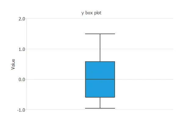
As we can see, the minimum is far away from the first quartile and the median. If we set the cleaning parameter to 0.6, Tukey’s method detects Point (A) as an outlier and removes it from the dataset.
Plotting the box plot for that variable again, we can notice that the outlier has been removed. As a consequence, the distribution of the data is now much better.
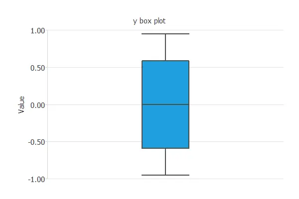
However, this univariate method has not detected Point (B), so we are not finished.
2. Multivariate method
Outliers do not need to be extreme values. Indeed, as we have seen with Point (B), the univariate method does not always work well. The multivariate approach attempts to address this by building a predictive model using all available data and removing instances with errors exceeding a given threshold.
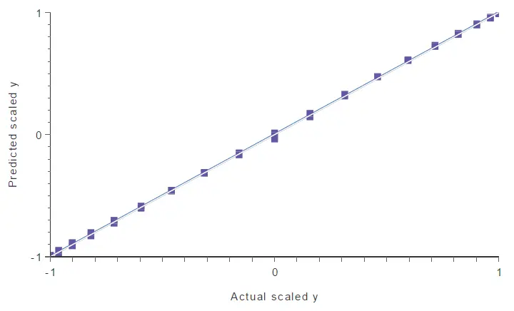
In this case, we have trained a neural network using all the available data (but Point (A), excluded by the univariate method). Then, we perform a linear regression analysis to obtain the following graph. The predicted values are plotted versus the real ones. The colored line indicates the best linear fit, and the grey line indicates a perfect fit.
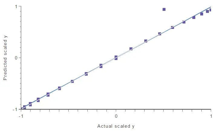
In the above chart, a point falls too far from the model. This point spoils the model, and therefore, it might be another outlier.
To find that point quantitatively, we can calculate the maximum error between the model’s outputs and the targets. The following table lists the five instances with maximum errors.
| Instance | Error | X | Y |
|---|---|---|---|
| 11 | 0.430 | 0.500 | 0.500 |
| 10 | 0.069 | 0.550 | 0.987 |
| 12 | 0.067 | 0.450 | 0.987 |
| 9 | 0.064 | 0.600 | 0.951 |
| 13 | 0.058 | 0.400 | 0.951 |
As we can notice, sample 11 has a significant error compared to the others. If we look at the linear regression chart, we see that this instance matches the point far from the model.
By selecting 20% of maximum error, this method identifies Point B as an outlier and cleans it from the data set. We can see that by performing a linear regression analysis again.
There are no more outliers in the data set, so the neural network’s generalization capabilities improve notably.
3. Minkowski error
Now, we will discuss an alternative method for handling outliers. Unlike the univariate and multivariate methods, it doesn’t detect or clean the outliers. Instead, it reduces the impact that outliers will have on the model.
The Minkowski error is a loss index that is less sensitive to outliers than the standard mean squared error.
The mean squared error raises each instance error to the square, making a too-big contribution of outliers to the total error,
$$mean\_squared\_error = \frac{\sum \left(outputs – targets\right)^2}{instances\_number}$$
The Minkowski error addresses this by raising each instance error to a power smaller than 2. This number is called the Minkowski parameter and reduces the contribution of outliers to the total error,
$$minkowski\_error = \frac{\sum\left(outputs – targets\right)^{minkowski\_parameter}}{instances\_number}$$
A typical value for the Minkowski parameter is 1.5.
For instance, if an outlier has an error of 10, the squared error for that instance is $(10^2=100)$, while the Minkowski error is $10^{1.5} = 31.62$.
To illustrate this method, we build two different neural networks using our dataset, which contains two outliers (A and B). The architecture selected for this network is 1:24:1. The loss index for the first neural network is the mean squared error. The loss index for the second neural network is the Minkowski error.
The neural network trained with the mean squared error is plotted in the following figure. As we can see, two outliers are spoiling the model.
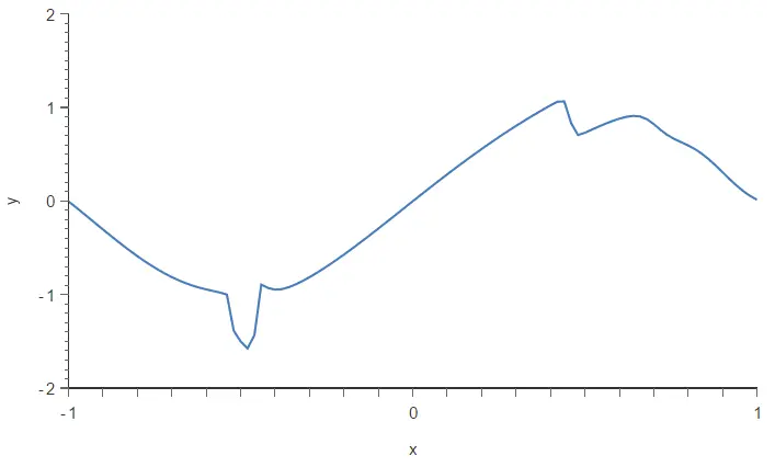
Now, we train the same neural network with the Minkowski error. The following figure depicts the resulting model.
As a result, the Minkowski error has made the training process less sensitive to outliers and has improved the quality of our model.
Conclusions
We have observed that outliers are a significant issue when building a predictive model. Indeed, they cause data scientists to achieve more unsatisfactory results than they could. We need practical methods to deal with those spurious points and remove them to resolve this issue.
In this article, we have seen 3 different methods for dealing with outliers: the univariate method, the multivariate method, and the Minkowski error. These methods are complementary, and we may need to try them all if our dataset contains many severe outliers.