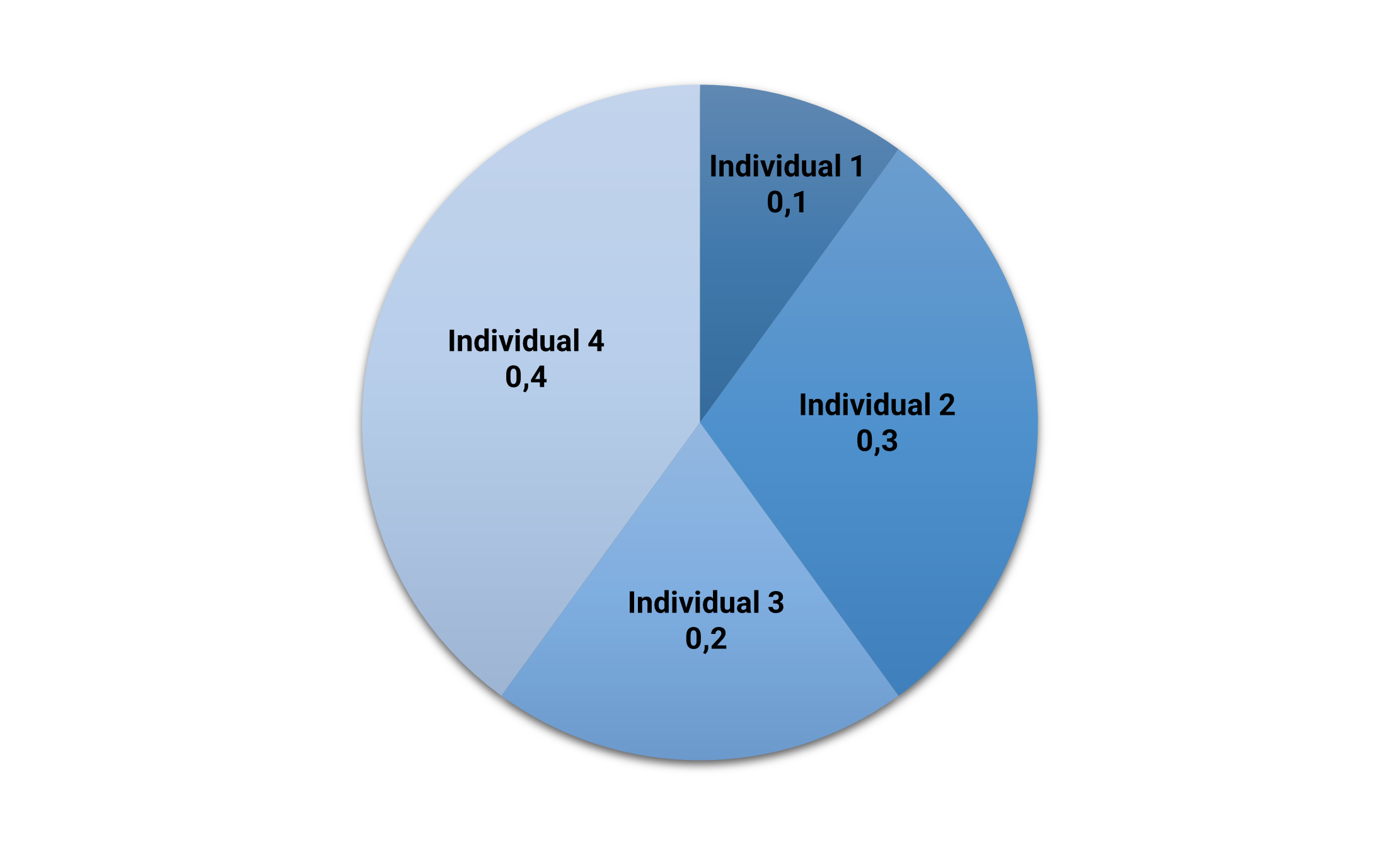
We can plot the above fitness values in a pie chart. Here, the area for each individual in the pie is proportional to its fitness.
The following picture shows the fitness pie.
3. Selection operator
After a fitness assignment has been performed, the selection operator chooses the individuals that recombine for the next generation.
The individuals most likely to survive are those more fitted to the environment. Therefore, the selection operator selects the individuals according to their fitness level. The number of selected individuals is N/2, being N the population size.
Elitist selection makes the fittest individuals survive directly for the next generation. The elitism size controls the number of directly selected individuals, and it is usually set to a small value (1,2,…).
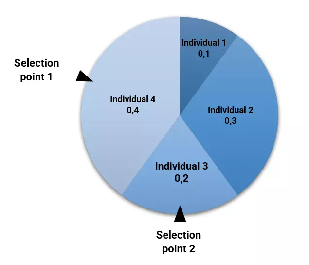
One of the most used selection methods is the roulette wheel. This method places all the individuals on a roulette, with areas proportional to their fitness, as we saw above. Then, it turns the roulette and selects the individuals at random. The corresponding individual is selected for recombination.
The following figure illustrates the selection process for our example.
4. Crossover operator
Once the selection operator has chosen half of the population, the crossover operator recombines the selected individuals to generate a new population.
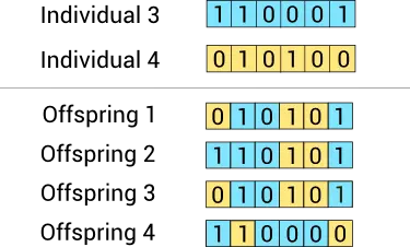
This operator picks two individuals randomly from the previously selected and combines their features to get four offspring for the new population until the new population is the same size as the old one.
The uniform crossover method decides whether each offspring’s features come from one parent or another.
The following figure illustrates the uniform crossover method for our example.
5. Mutation operator
The crossover operator can generate offspring that are very similar to the parents. This might cause a new generation with low diversity.
The mutation operator solves this problem by randomly changing the value of some features in the offspring.
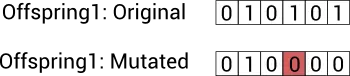
We generate a random number between 0 and 1 to decide if a feature is mutated. If the random number is lower than the mutation rate value, the operator flips that variable.
A standard value for the mutation rate is $dfrac{1}{m}$, where $m$ is the number of features. We mutate one feature of each individual (statistically) with that value.
The following image shows the mutation of one offspring of the new generation.
Process and results
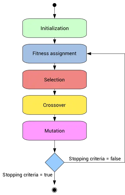
The whole fitness assignment, selection, recombination, and mutation process is repeated until a stopping criterion is satisfied.
Each generation will likely adapt more to the environment than the old one.
This chart shows the typical behavior of the mean selection error and the best selection error through generations. The example used is Breast Cancer Mortality example available in the blog.
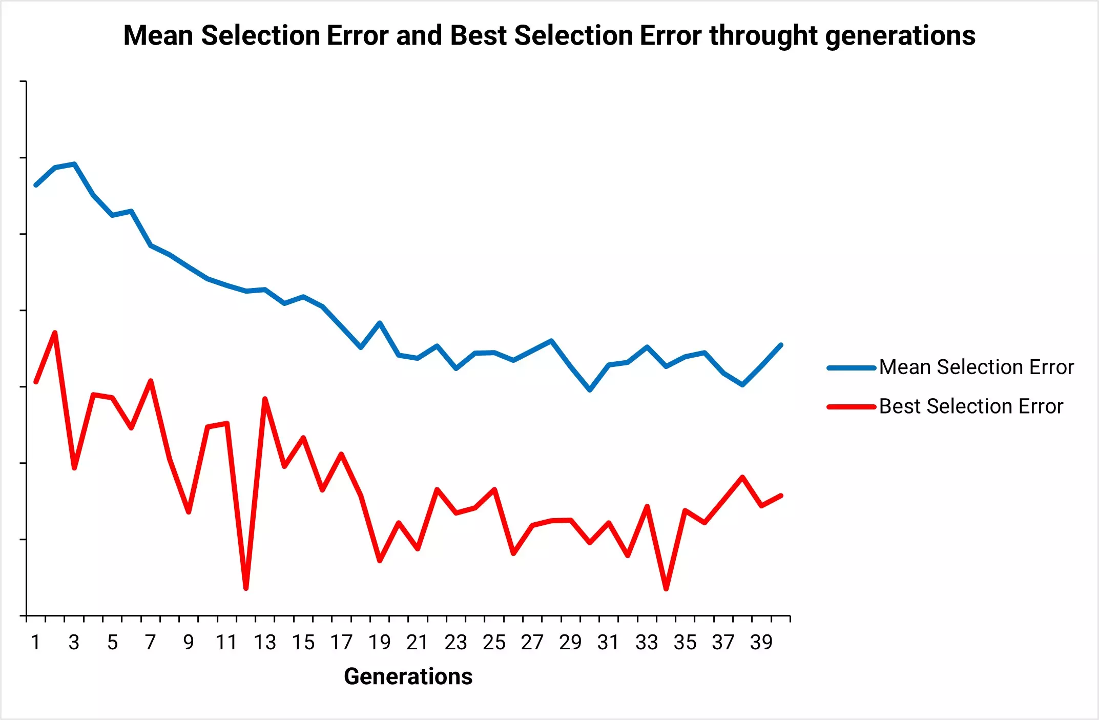
As we can see, the mean selection error at each generation converges to a minimum value.
The solution to this process is the best individual ever. This corresponds to the neural network with the smallest selection error among all those we have analyzed.
In our example, the best individual is the following:
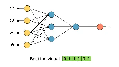
The above neural network is the selected one for our application.
Some disadvantages are:
- Genetic Algorithms might be costly in computational terms.
Indeed, the evaluation of each individual requires training a model. - These algorithms can take a long time to converge since they are stochastic.
In conclusion, genetic algorithms can select the best subset of our model’s variables but usually require much computation.
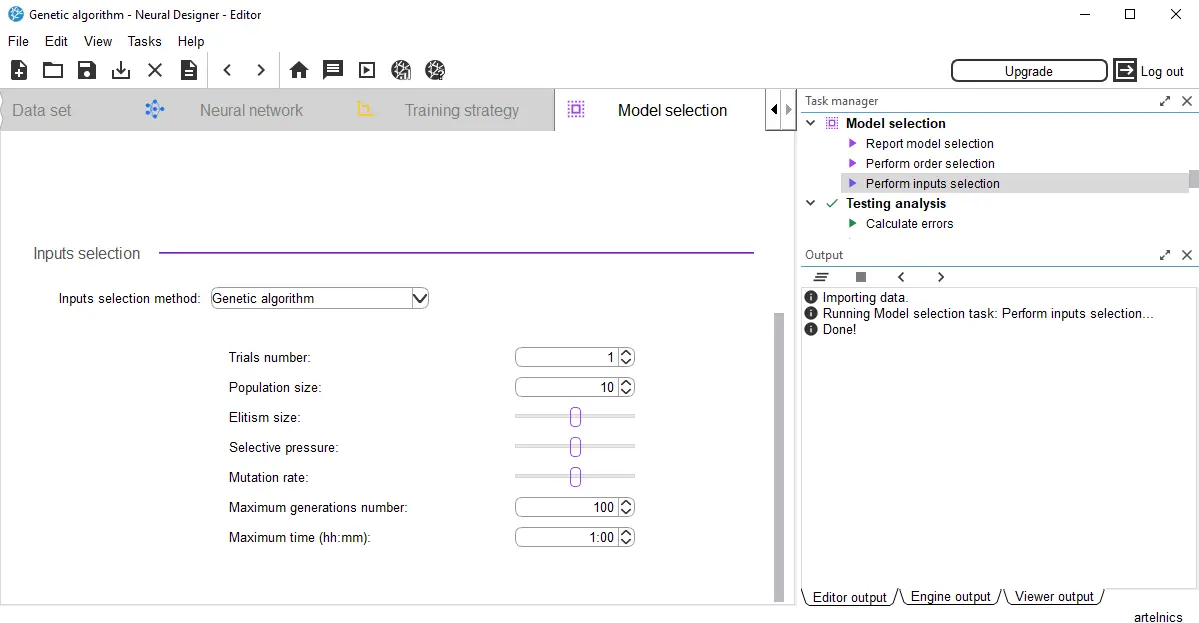
Neural Designer implements a more advanced genetic algorithm than the one described in this post.
You can find it in the input selection section in the model selection panel.