This example uses customer data from a bank to build a predictive model for identifying clients who are likely to churn. More specifically, the objective is to anticipate customer behavior before they decide to leave. By doing so, the bank can act proactively rather than reactively.
As we know, acquiring a new client is significantly more expensive than retaining an existing one. In fact, customer acquisition costs often exceed retention costs by a wide margin. Therefore, it is highly advantageous for banks to understand the factors that lead customers to leave the company. Moreover, early detection of dissatisfaction allows timely intervention.
In this context, Churn prevention enables financial institutions to design targeted loyalty programs and personalized retention campaigns. At the same time, it helps allocate marketing resources more efficiently. Consequently, banks can increase customer satisfaction, reduce attrition rates, and ultimately maintain long-term profitability.
Contents
- Application type.
- Data set.
- Neural network.
- Training strategy.
- Model selection.
- Testing analysis.
- Model deployment.
This example is solved with Neural Designer. To follow it step by step, you can use the free trial.
1. Application type
The variable to be predicted is binary (churn or loyal). Therefore this is a classification project.
The goal here is to model churn probability, conditioned on the customer features.
2. Data set
The data set contains information for creating our model. We need to configure three things here:
- Data source.
- Variables.
- Instances.
The data file bank_churn.csv contains 12 features about 10000 clients of the bank.
The features or variables are the following:
- customer_id, unused variable.
- credit_score, used as input.
- country, used as input.
- gender, used as input.
- age, used as input.
- tenure, used as input.
- balance, used as input.
- products_number, used as input.
- credit_card, used as input.
- active_member, used as input.
- estimated_salary, used as input.
- churn, used as the target. 1 if the client has left the bank during some period or 0 if he/she has not.
On the other hand, we randomly split the instances into training (60%), selection (20%), and testing (20%) subsets. In this way, the model learns from one portion of the data while we validate and evaluate it on unseen samples. As a result, this structure improves generalization and reduces overfitting risk.
Once we configure both the variables and the instance split, we can proceed with exploratory data analysis. At this stage, analyzing the dataset helps us better understand its structure before training the model.
In particular, the data distributions reveal the percentages of churn and loyal customers. Therefore, they provide insight into class balance. Moreover, this information allows us to anticipate potential modeling challenges related to imbalanced classes.
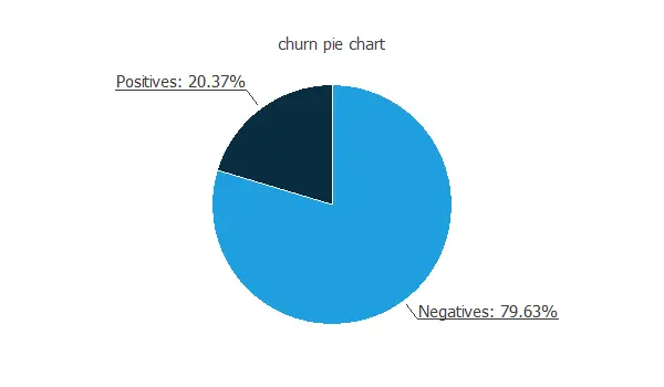
In this data set, the percentage of churn customers is about 20%.
The inputs-targets correlations might indicate which variables might be causing attrition.
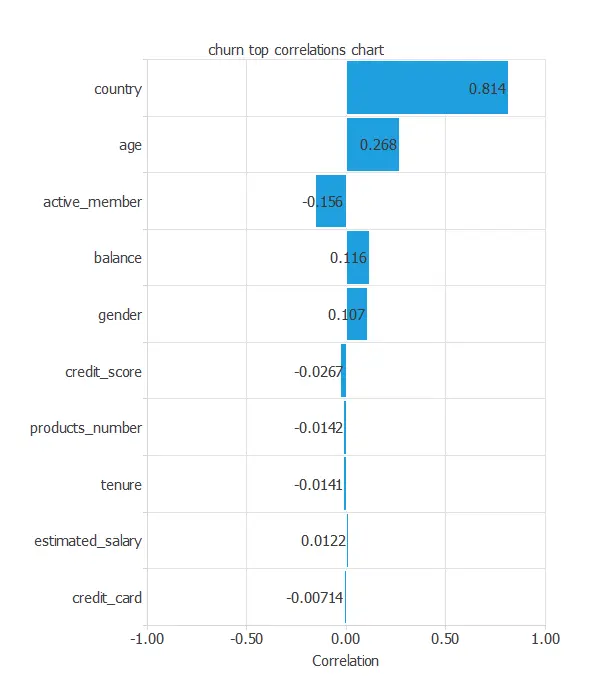
From the above chart, we can see that the country has a significant influence and that older customers have more probability of leaving the bank.
3. Neural network
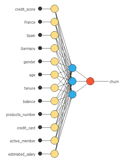
The second step is to choose a neural network to represent the classification function. For classification problems it is composed of:
For the scaling layer, the minimum and maximum scaling methods are set.
We set one perceptron layer, with 3 neurons as a first guess, having the logistic activation function.
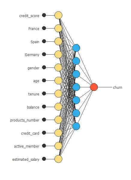
The next figure is a diagram for the neural network used in this example.
4. Training strategy
The training strategy is applied to the neural network to obtain the best possible performance. It is composed of two things:
- A loss index.
- An optimization algorithm.
The selected loss index is the weighted squared error with L2 regularization. The weighted squared error is helpful in applications where the targets are unbalanced. It gives a weight of 3.91 to churn customers and 1 to loyal customers.
The selected optimization algorithm is the quasi-Newton method.
The following chart shows how the training (blue) and selection (orange) errors decrease with the training epochs.
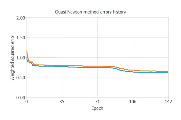
The final training and selection errors are training error = 0.621 WSE and selection error = 0.656 WSE, respectively. The following section will improve the generalization performance by reducing the selection error.
5. Model selection
Order selection is used to find the complexity of the neural network that optimizes the generalization performance. That is the number of neurons that minimize the error in the selection instances.
The following chart shows the training and selection errors for each different order after performing the incremental order method.
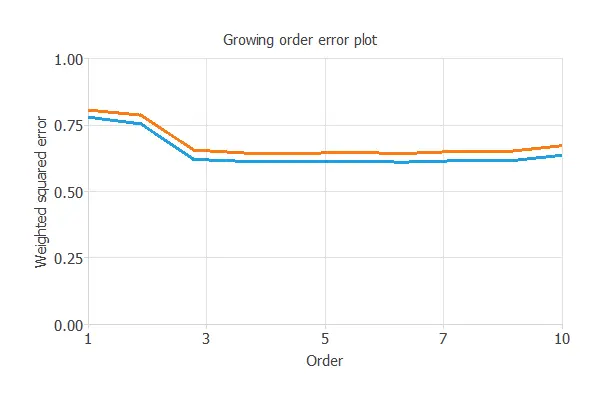
As the chart shows, the optimal number of neurons is 6, with selection error = 0.643.
Input selection (or feature selection) is used to find the set of inputs that produce the best generalization. The genetic algorithm has been applied here, but it does not reduce the selection error value, so we leave all input variables.
The following figure shows the final network architecture for this application.
6. Testing analysis
The next step is to perform an exhaustive testing analysis to validate the neural network’s predictive capabilities.
A good measure for the precision of a binary classification model is the ROC curve.
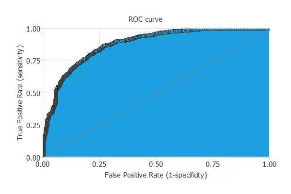
We are interested in the area under the curve (AUC). A perfect classifier would have an AUC=1, and a random one would have AUC=0.5. Our model has an AUC = 0.874, which is great.
We can also look at the confusion matrix. Next, we show the elements of this matrix for a decision threshold = 0.5.
| Predicted positive | Predicted negative | |
|---|---|---|
| Real positive | 305 (15%) | 80 (4%) |
| Real negative | 344 (17%) | 1271 (63%) |
From the above confusion matrix, we can calculate the following binary classification tests:
- Classification accuracy: 78.8% (ratio of correctly classified samples).
- Error rate: 21.2% (ratio of misclassified samples).
- Sensitivity: 79.2% (percentage of actual positive classified as positive).
- Specificity: 78.7% (percentage of actual negative classified as negative).
Now, we can simulate the performance of a retention campaign. For that, we use the cumulative gain chart.
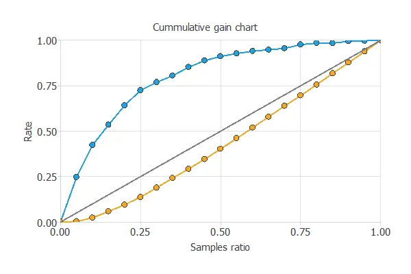
The above chart tells us that if we contact 25% of the customers with the highest chance of churn, we will reach 75% of the customers leaving the bank.
7. Model deployment
Once we have tested the churn model, we can use it to evaluate the probability of churn of our customers.
For instance, consider a customer with the following features:
- credit_score: 650
- country: France
- gender: Female
- age: 39
- tenure: 5
- balance: 76485
- products_number: 2
- credit_card: Yes
- active_member: No
- estimated_salary: 100000
The probability of churn for that customer is 38%.
We can export the mathematical expression of the neural network to any bank software to facilitate the work of the Retention Department. This expression is listed below.
scaled_credit_score = (credit_score-650.529)/96.6533;
scaled_France = 2*(France-0)/(1-0)-1;
scaled_Spain = (Spain-0.2477)/0.431698;
scaled_Germany = (Germany-0.2509)/0.433553;
scaled_gender = 2*(gender-0)/(1-0)-1;
scaled_age = (age-38.9218)/10.4878;
scaled_tenure = 2*(tenure-0)/(10-0)-1;
scaled_balance = (balance-76485.9)/62397.4;
scaled_products_number = (products_number-1.5302)/0.581654;
scaled_credit_card = 2*(credit_card-0)/(1-0)-1;
scaled_active_member = 2*(active_member-0)/(1-0)-1;
scaled_estimated_salary = 2*(estimated_salary-11.58)/(199992-11.58)-1;
y_1_1 = Logistic (0.848205+ (scaled_credit_score*-0.608944)+ (scaled_France*-0.261025)+ (scaled_Spain*0.412236)+ (scaled_Germany*-0.102466)+ (scaled_gender*-0.190523)+ (scaled_age*-5.79629)+ (scaled_tenure*-0.538913)+ (scaled_balance*-0.442531)+ (scaled_products_number*-2.72944)+ (scaled_credit_card*0.684301)+ (scaled_active_member*3.1411)+ (scaled_estimated_salary*1.5462));
y_1_2 = Logistic (-0.30529+ (scaled_credit_score*0.0542391)+ (scaled_France*-0.0197414)+ (scaled_Spain*-0.277012)+ (scaled_Germany*0.287529)+ (scaled_gender*-0.138025)+ (scaled_age*-1.67199)+ (scaled_tenure*-0.295799)+ (scaled_balance*-0.0519641)+ (scaled_products_number*-5.95291)+ (scaled_credit_card*-0.214941)+ (scaled_active_member*-1.43624)+ (scaled_estimated_salary*0.198904));
y_1_3 = Logistic (-0.0481312+ (scaled_credit_score*0.25511)+ (scaled_France*0.0844269)+ (scaled_Spain*0.108521)+ (scaled_Germany*-0.2049)+ (scaled_gender*0.125926)+ (scaled_age*0.0827378)+ (scaled_tenure*0.276278)+ (scaled_balance*-0.489973)+ (scaled_products_number*-0.776123)+ (scaled_credit_card*0.0203207)+ (scaled_active_member*0.525674)+ (scaled_estimated_salary*-0.17605));
y_1_4 = Logistic (1.52953+ (scaled_credit_score*-3.07592)+ (scaled_France*1.09842)+ (scaled_Spain*-1.4286)+ (scaled_Germany*0.153036)+ (scaled_gender*1.71313)+ (scaled_age*2.61432)+ (scaled_tenure*-3.80362)+ (scaled_balance*0.78056)+ (scaled_products_number*-1.88)+ (scaled_credit_card*-1.82242)+ (scaled_active_member*1.85776)+ (scaled_estimated_salary*1.40538));
y_1_5 = Logistic (-0.0116541+ (scaled_credit_score*0.144119)+ (scaled_France*-0.0170994)+ (scaled_Spain*0.0812705)+ (scaled_Germany*-0.0603271)+ (scaled_gender*-0.0485258)+ (scaled_age*-1.6572)+ (scaled_tenure*0.0583053)+ (scaled_balance*-0.135168)+ (scaled_products_number*-1.32794)+ (scaled_credit_card*0.0531906)+ (scaled_active_member*-1.13656)+ (scaled_estimated_salary*-0.128869));
y_1_6 = Logistic (-3.85516+ (scaled_credit_score*-0.0138554)+ (scaled_France*-0.753416)+ (scaled_Spain*-1.04647)+ (scaled_Germany*1.90095)+ (scaled_gender*0.0137635)+ (scaled_age*-0.191778)+ (scaled_tenure*0.343281)+ (scaled_balance*4.70446)+ (scaled_products_number*-6.3796)+ (scaled_credit_card*0.115022)+ (scaled_active_member*-0.153162)+ (scaled_estimated_salary*-0.0731349));
non_probabilistic_churn = Logistic (4.33579+ (y_1_1*-1.60163)+ (y_1_2*7.91345)+ (y_1_3*-6.65044)+ (y_1_4*-1.39552)+ (y_1_5*-5.56462)+ (y_1_6*-2.54043));
churn = probability(non_probabilistic_churn);

logistic(x){
   return 1/(1+exp(-x))
}

probability(x){
   if x < 0 return 0 else if x > 1
       return 1
   else
       return x
}