Classification of star types using machine learning

The main goal here is to design a model that makes proper classifications for the different star types.

Contents:

1. Application type.
2. Data set.
3. Neural network.
4. Training strategy.
5. Model selection.
6. Testing analysis.
7. Model deployment.

This example is solved with Neural Designer. To follow it step by step, you can use the free trial.

1. Application type

This is a classification project. Indeed, the variable to be predicted is categorical. The categories are Red Dwarf, Brown Dwarf, White Dwarf, Main Sequence, Supergiants, or Hypergiants.

The following image shows the star types mentioned:

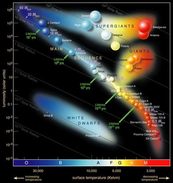
The classification is given according to different variables such as luminosity, radius, color, and other star characteristics. These variables are detailed in the following section.

2. Data set

The first step is to prepare the data set. This is the source of information for the classification problem. For that, we need to configure the following concepts:

• Data source.
• Variables.
• Instances.

The data source is the file Stars.csv. It contains the data for this example in comma-separated values (CSV) format. The number of columns is 7, and the number of rows is 240.

The variables are:

• Temperature: Temperature in Kelvin units.
• L: Luminosity in Sun luminosity units (L/L_0).
• R: Relative radius R/R_0 (R_0: Sun radius).
• A_M: Absolute Magnitude.
• Color: General color of spectrum.
• Spectral_Class: O,B,A,F,G,K,M.
• Type: Red Dwarf, Brown Dwarf, White Dwarf, Main Sequence, Supergiants, Hypergiants used as the target.

Note that neural networks work with numbers. In this regard, the categorical variable "class" is transformed into a numerical variable as follows:

• Red Dwarf: 1 0 0 0 0 0.
• Brown Dwarf: 0 1 0 0 0 0.
• White Dwarf: 0 0 1 0 0 0.
• Main Sequence: 0 0 0 1 0 0.
• Supergiants: 0 0 0 0 1 0.
• Hypergiants: 0 0 0 0 0 1.

The instances are divided into training, selection, and testing subsets. They represent 60% (144), 20% (48), and 20% (48) of the original instances, respectively, and are split at random.

We can calculate the distributions of all variables. The next figure is the pie chart for the star types.

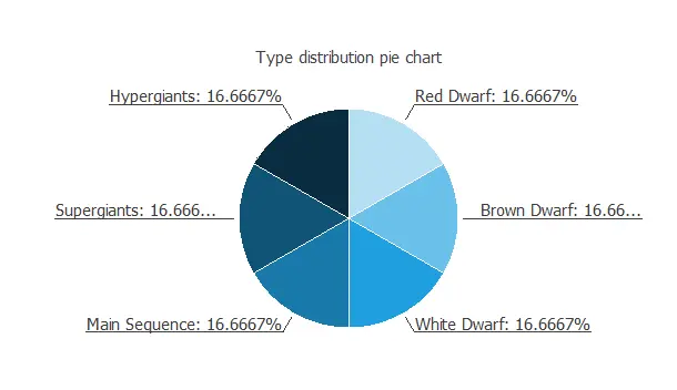
As we can see, the target is well-distributed.

3. Neural network

The second step is to choose a neural network. For classification problems, it is usually composed by:

• A scaling layer.
• A perceptron layer.
• A probabilistic layer.

The scaling layer contains the statistics on the inputs calculated from the data file and the method for scaling the input variables. Here the minimum-maximum method is set. Nevertheless, the mean-standard deviation method would produce very similar results.

The number of perceptron layers is 1. This perceptron layer has 22 inputs and 6 neurons.

The probabilistic layer allows the outputs to be interpreted as probabilities. This means that all the outputs are between 0 and 1, and their sum is 1. The softmax probabilistic method is used here.

The neural network has six outputs since the target variable contains six classes (Red Dwarf, Brown Dwarf, White Dwarf, Main Sequence, Supergiants, and Hypergiants).

4. Training strategy

The fourth step is to set the training strategy. It is composed of:

• Loss index.
• Optimization algorithm.

The loss index chosen for this application is the normalized squared error with L1 regularization.

The error term fits the neural network to the training instances of the data set. The regularization term makes the model more stable and improves generalization.

The optimization algorithm searches for the neural network parameters which minimize the loss index. The quasi-Newton method is chosen here.

The following chart shows how the training and selection errors decrease with the epochs during the training process.

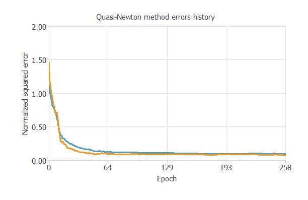
The final values are training error = 0.0912 NSE (blue), and selection error = 0.0735 NSE (orange).

5. Model selection

The objective of model selection is to find the network architecture with the best generalization properties. That is, the model which minimizes the error on the selected instances of the data set.

Order selection algorithms train several network architectures with a different number of neurons, and select that with the smallest selection error.

The incremental order method starts with a small number of neurons and increases the complexity at each iteration.

6. Testing analysis

The purpose of the testing analysis is to validate the generalization performance of the model. Here we compare the neural network outputs to the corresponding targets in the testing instances of the data set.

In the confusion matrix, the rows represent the targets (or real values) and the columns are the corresponding outputs (or predicted values). The diagonal cells show the correctly classified cases, and the off-diagonal cells show the misclassified cases.

7. Model deployment

The neural network is now ready to predict outputs for inputs that it has never seen. This process is called model deployment.

To classify any given star, we calculate the neural network outputs from the differents variables: temperature, luminosity, relative radius, absolute magnitude, color and spectral class. For example, if we introduce the following values for each input:

• Temperature: 10497.5 K.
• L (L/L_0): 107188.
• R (R/R_0): 237.2.
• A_M: 4.4.
• Color: Red.
• Spectral_Class: M.

The model predicts that the star belongs to each category with these probabilities.

• Probability of Red Dwarf: 1.3 %.
• Probability of Brown Dwarf: 81.1 %.
• Probability of White Dwarf: 0.2 %.
• Probability of Main Sequence: 7.3 %.
• Probability of Supergiants: 8.2 %.
• Probability of Hypergiants: 1.9 %.

The neural network would classify the star as a Brown Dwarf for this particular case since it has the highest probability.

The mathematical expression of the trained neural network is listed below.

scaled_Temperature = Temperature*(1+1)/(40000-(1939))-1939*(1+1)/(40000-1939)-1;

scaled_L = L*(1+1)/(849420-(7.999999798e-05))-7.999999798e-05*(1+1)/(849420-7.999999798e-05)-1;

scaled_R = R*(1+1)/(1948.5-(0.0083999997))-0.0083999997*(1+1)/(1948.5-0.0083999997)-1;

scaled_A_M = A_M*(1+1)/(20.05999947-(-11.92000008))+11.92000008*(1+1)/(20.05999947+11.92000008)-1;

scaled_Red = Red*(1+1)/(1-(0))-0*(1+1)/(1-0)-1;

scaled_Blue-White = Blue-White*(1+1)/(1-(0))-0*(1+1)/(1-0)-1;

scaled_White = White*(1+1)/(1-(0))-0*(1+1)/(1-0)-1;

scaled_Yellowish-White = Yellowish-White*(1+1)/(1-(0))-0*(1+1)/(1-0)-1;

scaled_Pale Yellow-Orange = Pale Yellow-Orange*(1+1)/(1-(0))-0*(1+1)/(1-0)-1;

scaled_Blue = Blue*(1+1)/(1-(0))-0*(1+1)/(1-0)-1;

scaled_Whitish = Whitish*(1+1)/(1-(0))-0*(1+1)/(1-0)-1;

scaled_Yellow-White = Yellow-White*(1+1)/(1-(0))-0*(1+1)/(1-0)-1;

scaled_Orange = Orange*(1+1)/(1-(0))-0*(1+1)/(1-0)-1;

scaled_Yellowish = Yellowish*(1+1)/(1-(0))-0*(1+1)/(1-0)-1;

scaled_Orange-Red = Orange-Red*(1+1)/(1-(0))-0*(1+1)/(1-0)-1;

scaled_M = M*(1+1)/(1-(0))-0*(1+1)/(1-0)-1;

scaled_B = B*(1+1)/(1-(0))-0*(1+1)/(1-0)-1;

scaled_A = A*(1+1)/(1-(0))-0*(1+1)/(1-0)-1;

scaled_F = F*(1+1)/(1-(0))-0*(1+1)/(1-0)-1;

scaled_O = O*(1+1)/(1-(0))-0*(1+1)/(1-0)-1;

scaled_K = K*(1+1)/(1-(0))-0*(1+1)/(1-0)-1;

scaled_G = G*(1+1)/(1-(0))-0*(1+1)/(1-0)-1;



perceptron_layer_0_output_0 = tanh[ -0.0117231 + (scaled_Temperature*0.00237329)+ (scaled_L*0.00604584)+ (scaled_R*0.00185487)+ (scaled_A_M*3.13471)+ (scaled_Red*-0.0339139)+ (scaled_Blue-White*0.228284)+ (scaled_White*0.315227)+ (scaled_Yellowish-White*0.432062)+ (scaled_Pale Yellow-Orange*0.00561356)+ (scaled_Blue*0.273381)+ (scaled_Whitish*0.00716272)+ (scaled_Yellow-White*0.00866841)+ (scaled_Orange*0.00625384)+ (scaled_Yellowish*0.0063531)+ (scaled_Orange-Red*0.0134212)+ (scaled_M*-0.141896)+ (scaled_B*0.45044)+ (scaled_A*0.125689)+ (scaled_F*0.0145472)+ (scaled_O*0.0100173)+ (scaled_K*0.00172927)+ (scaled_G*0.00502637) ];

perceptron_layer_0_output_1 = tanh[ 0.00515994 + (scaled_Temperature*0.000147072)+ (scaled_L*-0.00149089)+ (scaled_R*1.23767)+ (scaled_A_M*-0.700691)+ (scaled_Red*3.53748e-05)+ (scaled_Blue-White*-0.00451392)+ (scaled_White*-0.0738914)+ (scaled_Yellowish-White*-0.0202309)+ (scaled_Pale Yellow-Orange*-0.0412883)+ (scaled_Blue*-0.000217461)+ (scaled_Whitish*-0.0234267)+ (scaled_Yellow-White*-0.0125907)+ (scaled_Orange*-0.00391603)+ (scaled_Yellowish*-0.00626099)+ (scaled_Orange-Red*-0.0245549)+ (scaled_M*0.000219942)+ (scaled_B*-0.000499257)+ (scaled_A*-0.0182134)+ (scaled_F*-0.0242998)+ (scaled_O*0.00118038)+ (scaled_K*-0.0122634)+ (scaled_G*-0.0178582) ];

perceptron_layer_0_output_2 = tanh[ -0.00354958 + (scaled_Temperature*-0.668463)+ (scaled_L*0.494015)+ (scaled_R*-0.33068)+ (scaled_A_M*-0.787904)+ (scaled_Red*0.0856053)+ (scaled_Blue-White*0.00081301)+ (scaled_White*0.00497794)+ (scaled_Yellowish-White*0.00141669)+ (scaled_Pale Yellow-Orange*0.0013258)+ (scaled_Blue*0.556683)+ (scaled_Whitish*0.000844233)+ (scaled_Yellow-White*0.000371496)+ (scaled_Orange*0.00127982)+ (scaled_Yellowish*0.00558801)+ (scaled_Orange-Red*0.00249741)+ (scaled_M*0.118958)+ (scaled_B*0.151694)+ (scaled_A*0.000490191)+ (scaled_F*0.00207078)+ (scaled_O*-0.000891178)+ (scaled_K*0.000512244)+ (scaled_G*0.0034199) ];

perceptron_layer_0_output_3 = tanh[ 0.000901705 + (scaled_Temperature*-0.000137281)+ (scaled_L*0.00067225)+ (scaled_R*-0.00142935)+ (scaled_A_M*-0.00160211)+ (scaled_Red*-0.00514812)+ (scaled_Blue-White*7.49796e-05)+ (scaled_White*-0.00057408)+ (scaled_Yellowish-White*0.000354791)+ (scaled_Pale Yellow-Orange*-0.000849044)+ (scaled_Blue*-0.00010967)+ (scaled_Whitish*-0.000359372)+ (scaled_Yellow-White*-7.25229e-05)+ (scaled_Orange*0.000371288)+ (scaled_Yellowish*0.000325161)+ (scaled_Orange-Red*-0.00116547)+ (scaled_M*0.00171977)+ (scaled_B*-0.000358044)+ (scaled_A*0.000458903)+ (scaled_F*-0.000425171)+ (scaled_O*0.000584162)+ (scaled_K*0.000456646)+ (scaled_G*0.000430005) ];

perceptron_layer_0_output_4 = tanh[ 0.000295805 + (scaled_Temperature*-0.000538978)+ (scaled_L*-1.77957e-06)+ (scaled_R*-0.000733246)+ (scaled_A_M*6.6571e-05)+ (scaled_Red*0.000354727)+ (scaled_Blue-White*0.000297242)+ (scaled_White*-0.000202524)+ (scaled_Yellowish-White*2.57754e-05)+ (scaled_Pale Yellow-Orange*0.000143461)+ (scaled_Blue*0.00046088)+ (scaled_Whitish*-0.000777423)+ (scaled_Yellow-White*0.000628418)+ (scaled_Orange*0.000130731)+ (scaled_Yellowish*-0.000715591)+ (scaled_Orange-Red*-4.9299e-05)+ (scaled_M*-0.000976888)+ (scaled_B*0.0016078)+ (scaled_A*0.000429827)+ (scaled_F*0.000496293)+ (scaled_O*-0.000312369)+ (scaled_K*-0.000155917)+ (scaled_G*0.00169588) ];

perceptron_layer_0_output_5 = tanh[ -0.00044046 + (scaled_Temperature*-0.00149568)+ (scaled_L*0.000732599)+ (scaled_R*0.000238403)+ (scaled_A_M*-1.66479e-05)+ (scaled_Red*0.575044)+ (scaled_Blue-White*-0.0028659)+ (scaled_White*-0.000786949)+ (scaled_Yellowish-White*-0.000716665)+ (scaled_Pale Yellow-Orange*-0.000926854)+ (scaled_Blue*0.00143756)+ (scaled_Whitish*0.000418471)+ (scaled_Yellow-White*-5.28031e-06)+ (scaled_Orange*0.00105306)+ (scaled_Yellowish*-0.00161558)+ (scaled_Orange-Red*-0.000646812)+ (scaled_M*0.964901)+ (scaled_B*-0.000724226)+ (scaled_A*-0.000615297)+ (scaled_F*0.000599087)+ (scaled_O*0.000718622)+ (scaled_K*-0.00109337)+ (scaled_G*0.000665177) ];



    probabilistic_layer_combinations_0 = 0.000404313 +3.82639*perceptron_layer_0_output_0 -0.000721998*perceptron_layer_0_output_1 -0.000646157*perceptron_layer_0_output_2 +2.7772e-06*perceptron_layer_0_output_3 +0.000878223*perceptron_layer_0_output_4 +0.767679*perceptron_layer_0_output_5 

    probabilistic_layer_combinations_1 = -0.000773603 -0.00185322*perceptron_layer_0_output_0 +0.000664287*perceptron_layer_0_output_1 -0.0030646*perceptron_layer_0_output_2 -0.00678238*perceptron_layer_0_output_3 +0.00133339*perceptron_layer_0_output_4 +1.21104*perceptron_layer_0_output_5 

    probabilistic_layer_combinations_2 = 0.000845719 +3.42098*perceptron_layer_0_output_0 +0.000295546*perceptron_layer_0_output_1 +0.00031342*perceptron_layer_0_output_2 +0.0010623*perceptron_layer_0_output_3 -0.000204875*perceptron_layer_0_output_4 -2.00074*perceptron_layer_0_output_5 

    probabilistic_layer_combinations_3 = -0.000226988 -0.00207612*perceptron_layer_0_output_0 -0.000349768*perceptron_layer_0_output_1 -0.0120626*perceptron_layer_0_output_2 +0.000410198*perceptron_layer_0_output_3 -0.000237159*perceptron_layer_0_output_4 -1.42748*perceptron_layer_0_output_5 

    probabilistic_layer_combinations_4 = 0.00104541 +9.79289e-05*perceptron_layer_0_output_0 -0.235448*perceptron_layer_0_output_1 +4.56892*perceptron_layer_0_output_2 -0.000171369*perceptron_layer_0_output_3 -1.71108e-05*perceptron_layer_0_output_4 -0.000656543*perceptron_layer_0_output_5 

    probabilistic_layer_combinations_5 = 0.00446992 -0.0563862*perceptron_layer_0_output_0 +4.70687*perceptron_layer_0_output_1 +0.00203545*perceptron_layer_0_output_2 +3.00151e-06*perceptron_layer_0_output_3 +0.000353131*perceptron_layer_0_output_4 -9.31739e-05*perceptron_layer_0_output_5 

    

    sum_ = exp(probabilistic_layer_combinations_0 + exp(probabilistic_layer_combinations_1 + exp(probabilistic_layer_combinations_2 + exp(probabilistic_layer_combinations_3 + exp(probabilistic_layer_combinations_4 + exp(probabilistic_layer_combinations_5;



    Red Dwarf = exp(probabilistic_layer_combinations_0)/sum_;

    Brown Dwarf = exp(probabilistic_layer_combinations_1)/sum_;

    White Dwarf = exp(probabilistic_layer_combinations_2)/sum_;

    Main Sequence = exp(probabilistic_layer_combinations_3)/sum_;

    Supergiants = exp(probabilistic_layer_combinations_4)/sum_;

    Hypergiants = exp(probabilistic_layer_combinations_5)/sum_;

        

In conclusion, we have built a predictive model from which to determine the category of a star.

References:

• Kaggle. Star dataset to predict star types.

Related posts:

• Asteroid orbit classification.