This example aims to catalog different chemical biodegradability using machine learning.
QSAR (Quantitative Structure-Activity Relationships) models are currently being developed more frequently.
To construct the QSAR model, we leverage the explainable machine learning platform Neural Designer.
For those interested in a hands-on experience, a free trial lets you meticulously follow the process.
Contents
1. Application type
The variable to be predicted can have two values (ready or not ready biodegradable molecule).
Thus, this is a binary classification project. The goal here is to observe the correlation between different molecular descriptors and the biodegradability of a molecule.
2. Data set
Data source
The file biodegradation.csv contains 1055 samples of chemicals, each with 41 inputs, and one is a binary target.
Variables
This data set contains the following variables:
Constitutional descriptors
- nHM – Number of heavy atoms.
- C% – Percentage of carbon atoms.
- nCp – Number of terminal primary C(sp³).
- nO – Number of oxygen atoms.
- nN – Number of nitrogen atoms.
- nX – Number of halogen atoms.
Topological descriptors
- F01[N-N] – Frequency of N–N bonds at topological distance 1.
- F02[C-N] – Frequency of C–N bonds at topological distance 2.
- F03[C-N] – Frequency of C–N bonds at topological distance 3.
- F04[C-N] – Frequency of C–N bonds at topological distance 4.
- F03[C-O] – Frequency of C–O bonds at topological distance 3.
- nCIR – Number of circuits.
- LOC – Lopping centric index.
- TI2_L – Second Mohar index from Laplace matrix.
Functional group descriptors
- NssssC – Number of atoms of type ssssC.
- nCb – Number of substituted benzene C(sp²).
- nN-N – Number of N hydrazines.
- nArNO2 – Number of aromatic nitro groups.
- nCRX3 – Number of CRX₃ groups.
- nCrt – Number of ring tertiary C(sp³).
- nArCOOR – Number of aromatic esters.
- nHDon – Number of H-bond donor atoms (N and O).
- C-026 – Functional group descriptor (R–CX–R).
- N-073 – Functional groups: Ar₂NH / Ar₃N / Ar₂N–Al / R..N..R.
- B01[C-Br] – Presence/absence of C–Br at distance 1.
- B03[C-Cl] – Presence/absence of C–Cl at distance 3.
- B04[C-Br] – Presence/absence of C–Br at distance 4.
Electronic / E-State descriptors
- SdssC – Sum of dssC E-states.
- SdO – Sum of dO E-states.
- Me – Mean atomic Sanderson electronegativity (scaled on carbon).
- Mi – Mean first ionization potential (scaled on carbon).
Spectral / Eigenvalue-based descriptors
- SpMax_L – Leading eigenvalue from Laplace matrix.
- SM6_L – Spectral moment of order 6 from Laplace matrix.
- SpMax_A – Leading eigenvalue from adjacency matrix (Lovász–Pelikan index).
- SpMax_B(m) – Leading eigenvalue from Burden matrix weighted by mass.
- SM6_B(m) – Spectral moment of order 6 from Burden matrix weighted by mass.
- J_Dz(e) – Balaban-like index from Barysz matrix weighted by electronegativity.
- HyWi_B(m) – Hyper-Wiener-like index (log) from Burden matrix weighted by mass.
- SpPosA_B(p) – Normalized spectral positive sum from Burden matrix weighted by polarizability.
- Psi_i_1d – Intrinsic state pseudoconnectivity index (type 1d).
- Psi_i_A – Intrinsic state pseudoconnectivity index (type S average).
Target variable
RB_NRB – Biodegradability label:
1 = ready biodegradable
0 = not ready biodegradable.
Instances
Finally, the use of all instances is set.
Note that each instance contains a different chemical’s input and target variables.
Variables distributions
Also, we can calculate the distributions for all variables.
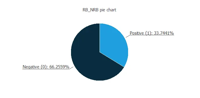
The figure below shows a pie chart of the dataset, comparing the proportion of biodegradable (positive) and non-biodegradable (negative) chemicals.
Input-target correlations
Finally, the input-target correlations might indicate which factors most influence biodegradability.
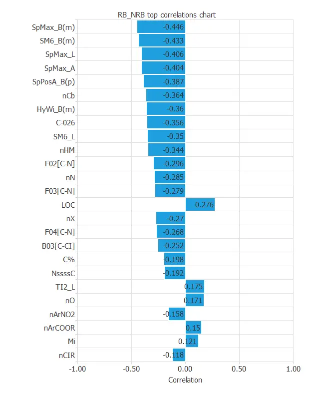
The most correlated variables are SpMax_B(m), SM6_B(m), SpMax_L, and SpMax_A, whose descriptions are above.
3. Neural network
The second step is to set a neural network representing the classification function. For this class of applications, the neural network is composed of:
- Scaling layer.
- Dense layer.
Scaling layer
The scaling layer contains the statistics on the inputs calculated from the data file and the method for scaling the input variables.
Here, the minimum and maximum methods have been set. Nevertheless, the mean and standard deviation method would produce very similar results.
Dense layer
For this example, we use a single dense layer. This layer has 41 inputs and 1 neuron.
Finally, we set the logistic activation function, as we want the predicted target variable to be binary.
4. Training strategy
The procedure used to carry out the learning process is called a training strategy.
The training strategy is applied to the neural network to obtain the best possible performance.
The type of training is determined by how the parameters in the neural network are adjusted.
This process is composed of two terms:
- A loss index.
- An optimization algorithm.
Loss index
The loss index is the mean squared error with L2 regularization. This is the default loss index for binary classification applications. The learning problem can be stated as finding a neural network that minimizes the loss index.
That is a neural network that fits the data set (error term) and does not oscillate (regularization term).
Optimization algorithm
The optimization algorithm that we use is the quasi-Newton method. This is also the standard optimization algorithm for this type of problem.
Training
The following chart shows how errors decrease with the iterations during training.
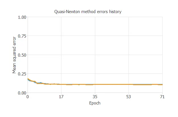
The final training and selection errors are training error = 0.108 WSE and selection error = 0.105 WSE, respectively.
5. Testing analysis
The objective of the testing analysis is to validate the generalization performance of the trained neural network.
To validate a classification technique, we need to compare the values provided by this technique to the observed values.
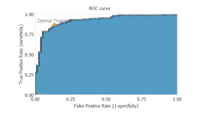
ROC curve
We can use the ROC curve as it is the standard testing method for binary classification projects.
Confusion matrix
The following table contains the elements of the confusion matrix.
This matrix shows the number of negative and positive predicted values versus the real ones.
| Predicted positive | Predicted negative | |
|---|---|---|
| Real positive | 59(28%) | 14(6.6%) |
| Real negative | 15(7.1%) | 123(58.3%) |
As we can see, the model correctly predicts 182 instances (86.3%) and misclassifies 29 (13.7%).
Note that most of our chemical data indicate that they are not readily biodegradable.
Binary classification metrics
The binary classification tests are parameters for measuring the performance of a classification problem with two classes:
- Accuracy (ratio of instances correctly classified): 86.3%
- Error (ratio of instances misclassified): 13.7%
- Sensitivity (ratio of real positives which the model predicts as positives): 86.3%
- Specificity (ratio of real negatives which the model predicts as negatives): 86.2%
6. Model deployment
Once we test the neural network’s generalization performance, we can save the neural network for future use in the so-called model deployment mode.
We can predict whether a chemical molecule is biodegradable by calculating the neural network outputs.
For that, we need to know the input variables for them.
We can export the mathematical expression of the neural network, which takes input variables to produce output variables, specifically to predict biodegradability.
This classification model propagates the information through the scaling, perceptron, and probabilistic layers.
Conclusions
References
- We have obtained the data for this problem from the UCI Machine Learning Repository.
- Mansouri, K., Ringsted, T., Ballabio, D., Todeschini, R., Consonni, V. (2013). Quantitative Structure-Activity Relationship models for ready biodegradability of chemicals. Journal of Chemical Information and Modeling, 53, 867-878.