
In this example, we develop a machine learning model to predict power generation at a solar plant located in Berkeley, CA.
We utilize various environmental conditions, including temperature, humidity, wind speed, and others.
Solar power is a free and clean alternative to traditional fossil fuels. However, the efficiency of solar cells is not as high as it could be nowadays.
Therefore, selecting the ideal conditions for its installation is critical to maximizing energy output. Knowing certain environmental conditions, we aim to predict the power output for a specific array of solar power generators.
This example is solved with Neural Designer. You can use the free trial to understand how the solution is achieved step by step.
Contents
- Application type.
- Data set.
- Neural network.
- Training strategy.
- Model selection.
- Testing analysis.
- Model deployment.
1. Application type
2. Data set
The first step is to prepare the dataset, which is the source of information for the approximation problem.
We have downloaded the raw data from Kaggle.
To achieve optimal results, we have processed this dataset.
Variables
Input variables
- distance_to_solar_noon – Distance to solar noon (radians).
- temperature – Daily average temperature (°C).
- wind_direction – Daily average wind direction (°; 0–360).
- wind_speed – Daily average wind speed (m/s).
- sky_cover – Cloud cover (0 = clear, 4 = fully covered).
- visibility – Visibility (km).
- humidity – Relative humidity (%).
- average_wind_speed – 3-hour average wind speed (m/s).
- average_pressure – 3-hour average barometric pressure (inHg).
Target variables
power_generated – Power generated in each 3-hour period (J).
Instances
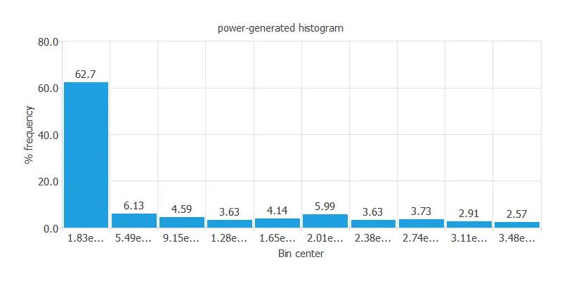
Distributions
Calculating the data distributions helps us verify the accuracy of the available information and detect anomalies.
Input-target correlations
It is also interesting to look for dependencies between a single input and a single target variable.
To do that, we can plot an input-target correlations chart.

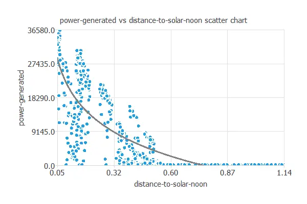
In this case, the highest correlation is with the distance to solar noon (the solar plant generates the closer to solar noon, the more power).
Scatter charts
Next, we plot a scatter chart for the most significant correlations for our target variable.
3. Neural network
The second step is to build a neural network that represents the approximation function. Approximation models usually contain the following layers:
- Scaling layer.
- Perceptron layers.
- Unscaling layer.
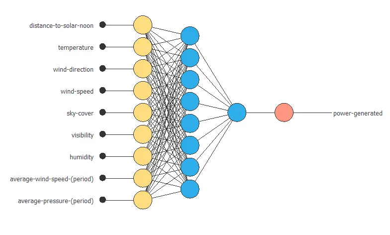
The neural network has nine inputs (distance to solar noon, temperature, wind direction, wind speed, sky cover, visibility, humidity, average wind speed (period), and average pressure (period)) and one output (power generated).
Scaling layer
The scaling layer contains the statistics of the inputs. We use the automatic setting for this layer to accommodate the best scaling technique for our data.
Desnse layers
We use 2 perceptron layers here.
The hidden perceptron layer has 9 inputs, 3 neurons, and a hyperbolic tangent activation function.
The output perceptron layer has 3 inputs, 1 neuron, and a linear activation function.
Unscaling layer
The unscaling layer contains the statistics of the outputs. We use the automatic method as before.
Neural network graph
The following graph represents the neural network for this example.

4. Training strategy
The fourth step is to select an appropriate training strategy.
It is composed of two concepts:
- Loss index.
- Optimization algorithm.
Loss index
The loss index defines what the neural network will learn. It is composed of an error term and a regularization term.
The error term we choose is the normalized squared error. It divides the squared error between the neural network outputs and the data set’s targets by its normalization coefficient. If the normalized squared error is 1, the neural network predicts the data ‘in the mean’, while a value of 0 means a perfect data prediction. This error term has no parameters to set.
The regularization term is the L2 regularization. It controls the neural network’s complexity by reducing the values of the parameters. We use a weak weight for this regularization term.
Optimization algorithm
The optimization algorithm is responsible for searching for the neural network parameters that minimize the loss index.
Here, we chose the quasi-Newton method as an optimization algorithm.
Training
The following chart shows how the training error (blue) and the selection error (orange) decrease with the number of epochs during training.
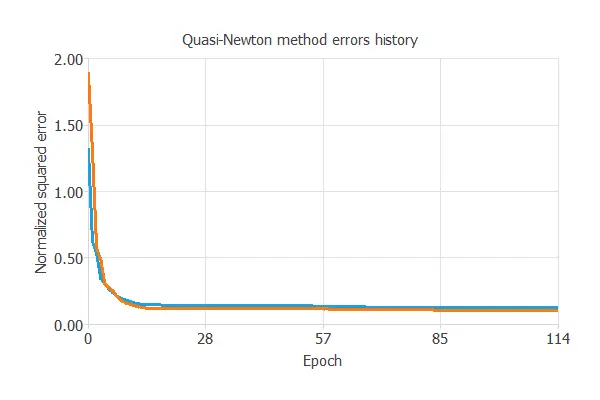
The final values are training error = 0.121 NSE and selection error = 0.122 NSE, respectively.
5. Model selection
The objective of model selection is to find the network architecture with the best generalization properties.
We aim to reduce the final selection error obtained previously (0.122 NSE).
Neuron selection
The best selection error is achieved using a model with the most appropriate complexity to produce a good data fit.
Order selection algorithms are responsible for finding the optimal number of perceptrons in the neural network.
The following chart shows the results of the incremental order algorithm.
The blue line shows training error and the orange line shows selection error, both versus the number of neurons.
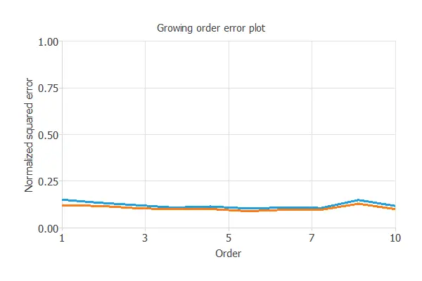
As we can see, the final training error continuously decreases with the number of neurons. However, the final selection error takes a minimum value at some point.
The optimal number of neurons is 8, corresponding to a selection error of 0.089 NSE.
Neural network graph
The following figure shows the optimal network architecture for this application.
6. Testing analysis
The purpose of the testing analysis is to validate the generalization capabilities of the neural network.
We use the testing instances in the data set, which have never been used before.
Goodnes-of-fit
A standard testing method in approximation applications is to perform a linear regression analysis between the predicted and the real values.
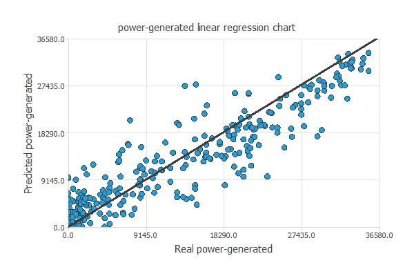
For a perfect fit, the correlation coefficient R2 would be 1. With R2 = 0.951, the neural network accurately predicts the testing data.
7. Model deployment
In the model deployment phase, the neural network predicts outputs for inputs it has not seen before.
Neural network outputs
We can calculate the neural network outputs for a given set of inputs:
- distance_to_solar_noon: 0.503 radians.
- temperature: 58.468ºC.
- wind_direction: 24.953º.
- wind_speed: 10.097 m/s.
- sky_cover: 1.988 over 4.
- visibility: 9.558 km.
- humidity: 73.524%.
- average-wind-speed-(period): 10.136 m/s.
- average_pressure_(period): 30.062 mercury inches.
The predicted output for these input values is the following:
- power_generated: 3012.461 Jules per 3-hour period.
Directional outputs
Directional outputs plot the neural network outputs through some reference points.
The next list shows the reference point for the plots.
- distance_to_solar_noon: 0.503 radians.
- temperature: 58.468ºC.
- wind_direction: 24.953º.
- wind_speed: 10.097 m/s.
- sky_cover: 1.988 over 4.
- visibility: 9.558 km.
- humidity: 73.524%.
- average_wind_speed: 10.136 m/s.
- average_pressure: 30.062 mercury inches.
We can see here how the distance to solar noon affects the power generated:

8. Video tutorial
References
Ph.D. candidate Alexandra Constantin compiled the data.