In this example, we will detect anomalies in beach water quality by using machine learning and auto association techniques. This approach has the potential to improve the accuracy of beach water quality forecasts, allowing for more informed decision-making by beach managers and the public.

Beaches are a popular destination for many people, whether for swimming, surfing, sunbathing, or simply enjoying the scenery.

However, the quality of the water at a beach can have a significant impact on the health and safety of beachgoers. A neural network can learn the patterns and correlations within a dataset. 

Contents

  1. Application type.
  2. Data set.
  3. Neural network.
  4. Model deployment.

This example is solved with Neural Designer. To follow it step by step, you can use the free trial.

Application type

In this application type, the outputs are the same as the inputs. Therefore, this is an auto association problem.

The goal of this auto association problem is to determine water quality levels by inputting historical data on these environmental factors and corresponding water quality measurements.

Data set

The first step is to prepare the data set, which is the source of information for this auto association problem. It is composed of:

Data source

The data source is the file beach-water-quality.csv. It contains the data for this example in comma-separated values (CSV) format. The number of columns is 6, and the number of rows is 11568.

The columns in the data set are this example’s variables. Because it is an auto association problem, all of the variables are input variables
as well as output variables or target variables.

All the variables in this example are numerical, and they are the following:

  • water_temperature.
  • turbidity.
  • transducer_depth.
  • wave_height.
  • wave_period.
  • battery_life.

The rows from the data set are the samples that we use for training and testing. Training samples are used to build different models with different topologies, and testing samples are used to validate the performance of the model.

The following pie chart details the uses of all cases in the data set.
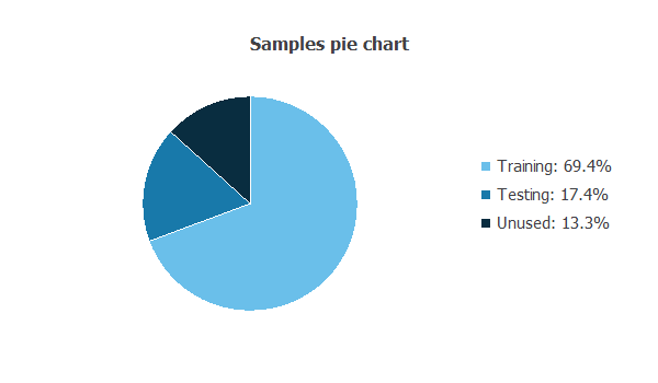
The following pie chart details the uses of all cases in the data set used in the machine learning model to detect anomalies in beach water quality. We have a 69.4% for training, 17.4% for testing and 13.3% for unused.

Out of the 11568 samples (rows), 8023 samples (69.4%) are used for training, and 2011 samples (17.4%) are used for testing. The remaining 1534 samples are unused variables.

Statistics

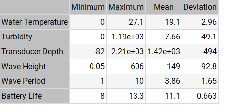
The bare statistics provide valuable information when designing a model. The table below shows the minimums, maximums, means, and standard deviations of all variables in our data set.

Neural network

The neural network will output all of the target variables as a function of the input variables that we described in the previous section.

For this auto association example, the neural network is composed of:

  • A scaling layer.
  • A mapping layer.
  • A bottleneck layer.
  • A demapping layer.
  • An output layer.
  • An unscaling layer.

The scaling layer contains the statistics on the input calculated from the data file and the method for scaling the input variables. Here, the mean and standard deviation scaling methods are set.

In neural network architecture, a mapping layer refers to a layer of neurons that perform a nonlinear transformation on the input data. The mapping layer is responsible for taking the input data and mapping it to a new space where it can be more easily separated by subsequent layers.

The mapping layer is followed by a bottleneck layer and a demapping layer. The bottleneck layer is typically located in the middle of the network, and it is used to reduce the dimensionality of the feature maps, thereby compressing the information contained in the data.

The demapping layer performs an inverse operation to the mapping layer.

In this problem, the hyperbolic tangent activation function is used as the activation in the mapping and demapping layers and the linear activation function in the bottleneck and output layers.

The following image depicts the neural network architecture of this auto association problem.

Neural network for the machine learning model used to dectect anomalies in the beach water quality.

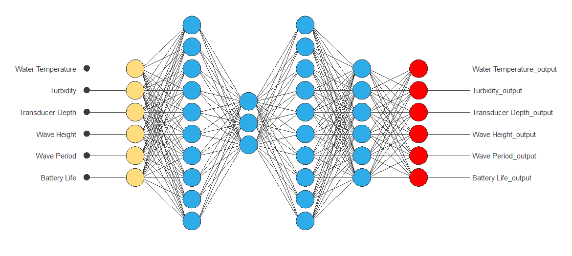
The yellow circles represent scaling neurons. The blue circles represent the mapping layer, the bottleneck layer, the demapping layer, and the output layer in that order. The red circles represent unscaling neurons.

As we can see, there are 6 neurons in the scaling, output, and unscaling layers. This is because, in auto-associative neural networks, we want to learn to replicate the input data as closely as possible. There are 10 neurons in the mapping and demapping layers and 3 neurons in the bottleneck layer.

Model deployment

Once we have tested the neural network’s generalization performance, we can save it for future use with the model deployment function.

The mathematical expression represented by the neural network is written below.

scaled_Water_Temperature = (Water_Temperature-19.07550049)/2.963890076;
scaled_Turbidity = (Turbidity-7.660490036)/49.14889908;
scaled_Transducer_Depth = (Transducer_Depth-1417.459961)/493.9230042;
scaled_Wave_Height = (Wave_Height-148.6869965)/92.75859833;
scaled_Wave_Period = (Wave_Period-3.864459991)/1.645190001;
scaled_Battery_Li_fe = (Battery_Li_fe-11.07509995)/0.6634060144;

mapping_layer_output_0 = tanh( 1.46985 + (scaled_Water_Temperature*-0.0372088) + (scaled_Turbidity*-0.109603) + (scaled_Transducer_Depth*0.595938) + (scaled_Wave_Height*0.000698271) + (scaled_Wave_Period*-0.0488589) + (scaled_Battery_Li_fe*-0.00409911) );
mapping_layer_output_1 = tanh( 0.794064 + (scaled_Water_Temperature*0.197965) + (scaled_Turbidity*-0.0461576) + (scaled_Transducer_Depth*-0.0173141) + (scaled_Wave_Height*-0.0193869) + (scaled_Wave_Period*-0.0433049) + (scaled_Battery_Li_fe*0.02329) );
mapping_layer_output_2 = tanh( 0.679954 + (scaled_Water_Temperature*-0.187078) + (scaled_Turbidity*0.109113) + (scaled_Transducer_Depth*0.0310535) + (scaled_Wave_Height*0.0661584) + (scaled_Wave_Period*0.237889) + (scaled_Battery_Li_fe*-0.172827) );
mapping_layer_output_3 = tanh( -0.23444 + (scaled_Water_Temperature*-0.1106) + (scaled_Turbidity*-0.0265759) + (scaled_Transducer_Depth*-0.10726) + (scaled_Wave_Height*0.241238) + (scaled_Wave_Period*-0.0700205) + (scaled_Battery_Li_fe*-0.151417) );
mapping_layer_output_4 = tanh( -0.181624 + (scaled_Water_Temperature*0.113892) + (scaled_Turbidity*0.0331958) + (scaled_Transducer_Depth*-0.0529271) + (scaled_Wave_Height*0.228245) + (scaled_Wave_Period*-0.14867) + (scaled_Battery_Li_fe*0.0240132) );
mapping_layer_output_5 = tanh( 0.117632 + (scaled_Water_Temperature*-0.102503) + (scaled_Turbidity*-0.047737) + (scaled_Transducer_Depth*0.0128806) + (scaled_Wave_Height*0.0718966) + (scaled_Wave_Period*0.189969) + (scaled_Battery_Li_fe*0.0366286) );
mapping_layer_output_6 = tanh( -0.430236 + (scaled_Water_Temperature*0.103023) + (scaled_Turbidity*0.0849286) + (scaled_Transducer_Depth*0.0699436) + (scaled_Wave_Height*0.0682575) + (scaled_Wave_Period*0.307539) + (scaled_Battery_Li_fe*-0.0100997) );
mapping_layer_output_7 = tanh( 2.03485 + (scaled_Water_Temperature*-0.0500029) + (scaled_Turbidity*-0.052288) + (scaled_Transducer_Depth*1.06615) + (scaled_Wave_Height*0.0327393) + (scaled_Wave_Period*-0.052899) + (scaled_Battery_Li_fe*-0.0495735) );
mapping_layer_output_8 = tanh( 0.145849 + (scaled_Water_Temperature*0.0204336) + (scaled_Turbidity*0.0216357) + (scaled_Transducer_Depth*0.0233445) + (scaled_Wave_Height*0.133806) + (scaled_Wave_Period*-0.0289289) + (scaled_Battery_Li_fe*0.0482352) );
mapping_layer_output_9 = tanh( -0.537646 + (scaled_Water_Temperature*0.0475645) + (scaled_Turbidity*0.013785) + (scaled_Transducer_Depth*-0.0462226) + (scaled_Wave_Height*0.00487573) + (scaled_Wave_Period*-0.0753554) + (scaled_Battery_Li_fe*-0.183019) );

bottle_neck_layer_output_0 = ( 0.421369 + (mapping_layer_output_0*0.0654674) + (mapping_layer_output_1*0.475325) + (mapping_layer_output_2*0.402376) + (mapping_layer_output_3*-0.68093) + (mapping_layer_output_4*-0.476745) + (mapping_layer_output_5*-0.423164) + (mapping_layer_output_6*0.13732) + (mapping_layer_output_7*-1.31888) + (mapping_layer_output_8*-0.769477) + (mapping_layer_output_9*0.955384) );
bottle_neck_layer_output_1 = ( 0.248485 + (mapping_layer_output_0*-0.246718) + (mapping_layer_output_1*0.320763) + (mapping_layer_output_2*0.353968) + (mapping_layer_output_3*0.32952) + (mapping_layer_output_4*0.516389) + (mapping_layer_output_5*-1.18656) + (mapping_layer_output_6*0.445537) + (mapping_layer_output_7*1.60113) + (mapping_layer_output_8*1.08479) + (mapping_layer_output_9*0.420113) );
bottle_neck_layer_output_2 = ( -0.827803 + (mapping_layer_output_0*1.28316) + (mapping_layer_output_1*1.23347) + (mapping_layer_output_2*-0.900268) + (mapping_layer_output_3*0.477456) + (mapping_layer_output_4*0.220512) + (mapping_layer_output_5*1.26906) + (mapping_layer_output_6*-0.929525) + (mapping_layer_output_7*0.359401) + (mapping_layer_output_8*0.144748) + (mapping_layer_output_9*0.330872) );

demapping_layer_output_0 = tanh( 0.0735414 + (bottle_neck_layer_output_0*0.120889) + (bottle_neck_layer_output_1*-0.19531) + (bottle_neck_layer_output_2*-0.347805) );
demapping_layer_output_1 = tanh( -0.906261 + (bottle_neck_layer_output_0*0.815783) + (bottle_neck_layer_output_1*0.677409) + (bottle_neck_layer_output_2*0.0232295) );
demapping_layer_output_2 = tanh( 0.242961 + (bottle_neck_layer_output_0*0.236328) + (bottle_neck_layer_output_1*-0.262859) + (bottle_neck_layer_output_2*0.141903) );
demapping_layer_output_3 = tanh( 1.4692 + (bottle_neck_layer_output_0*0.430476) + (bottle_neck_layer_output_1*-0.207925) + (bottle_neck_layer_output_2*0.630849) );
demapping_layer_output_4 = tanh( -0.355235 + (bottle_neck_layer_output_0*-0.257279) + (bottle_neck_layer_output_1*-0.163889) + (bottle_neck_layer_output_2*0.152867) );
demapping_layer_output_5 = tanh( 0.0310841 + (bottle_neck_layer_output_0*2.27302) + (bottle_neck_layer_output_1*-2.48378) + (bottle_neck_layer_output_2*-1.2984) );
demapping_layer_output_6 = tanh( -0.591744 + (bottle_neck_layer_output_0*0.580596) + (bottle_neck_layer_output_1*0.177818) + (bottle_neck_layer_output_2*0.47668) );
demapping_layer_output_7 = tanh( 0.025192 + (bottle_neck_layer_output_0*0.053212) + (bottle_neck_layer_output_1*1.71179) + (bottle_neck_layer_output_2*-2.34008) );
demapping_layer_output_8 = tanh( -1.52904 + (bottle_neck_layer_output_0*0.487859) + (bottle_neck_layer_output_1*-0.869553) + (bottle_neck_layer_output_2*1.91685) );
demapping_.layer_output_9 = tanh( -1.0758 + (bottle_neck_layer_output_0*-1.17594) + (bottle_neck_layer_output_1*-0.70896) + (bottle_neck_layer_output_2*-0.422137) );

output_layer_output_0 = ( -1.56952 + (demapping_layer_output_0*-0.559567) + (demapping_layer_output_1*-0.72369) + (demapping_layer_output_2*-0.941552) + (demapping_layer_output_3*-0.742017) + (demapping_layer_output_4*-0.819629) + (demapping_layer_output_5*0.61267) + (demapping_layer_output_6*1.9023) + (demapping_layer_output_7*1.28431) + (demapping_layer_output_8*0.891696) + (demapping_layer_output_9*-3.37984) );
output_layer_output_1 = ( 3.09887 + (demapping_layer_output_0*1.83668) + (demapping_layer_output_1*2.85019) + (demapping_layer_output_2*-3.01807) + (demapping_layer_output_3*-3.61545) + (demapping_layer_output_4*-2.32326) + (demapping_layer_output_5*-0.266023) + (demapping_layer_output_6*-3.8381) + (demapping_layer_output_7*-1.04943) + (demapping_layer_output_8*1.15035) + (demapping_layer_output_9*-1.12836) );
output_layer_output_2 = ( -1.18246 + (demapping_layer_output_0*0.429782) + (demapping_layer_output_1*0.320502) + (demapping_layer_output_2*-0.478118) + (demapping_layer_output_3*0.11112) + (demapping_layer_output_4*0.750794) + (demapping_layer_output_5*-1.54704) + (demapping_layer_output_6*-0.014775) + (demapping_layer_output_7*-0.0761109) + (demapping_layer_output_8*-0.360334) + (demapping_layer_output_9*-0.0907909) );
output_layer_output_3 = ( 1.34675 + (demapping_layer_output_0*-2.34536) + (demapping_layer_output_1*-0.953547) + (demapping_layer_output_2*-3.48551) + (demapping_layer_output_3*-0.224114) + (demapping_layer_output_4*1.46921) + (demapping_layer_output_5*2.87561) + (demapping_layer_output_6*-0.410865) + (demapping_layer_output_7*0.657503) + (demapping_layer_output_8*-0.632641) + (demapping_layer_output_9*0.51721) );
output_layer_output_4 = ( -1.28316 + (demapping_layer_output_0*1.52013) + (demapping_layer_output_1*-1.95027) + (demapping_layer_output_2*2.36864) + (demapping_layer_output_3*-0.339328) + (demapping_layer_output_4*-0.0368388) + (demapping_layer_output_5*-1.7285) + (demapping_layer_output_6*-1.09654) + (demapping_layer_output_7*1.5488) + (demapping_layer_output_8*-0.740122) + (demapping_layer_output_9*-0.0832852) );
output_layer_output_5 = ( 0.88104 + (demapping_layer_output_0*0.694486) + (demapping_layer_output_1*-1.81261) + (demapping_layer_output_2*-0.418974) + (demapping_layer_output_3*-0.526685) + (demapping_layer_output_4*0.297614) + (demapping_layer_output_5*-0.0588199) + (demapping_layer_output_6*-1.113) + (demapping_layer_output_7*0.332893) + (demapping_layer_output_8*2.87013) + (demapping_layer_output_9*-1.0765) );

Water_Temperature_output=output_layer_output_0*2.963890076+19.07550049;
Turbidity_output=output_layer_output_1*49.14889908+7.660490036;
Transducer_Depth_output=output_layer_output_2*493.9230042+1417.459961;
Wave_Height_output=output_layer_output_3*92.75859833+148.6869965;
Wave_Period_output=output_layer_output_4*1.645190001+3.864459991;
Battery_Li_fe_output=output_layer_output_5*0.6634060144+11.07509995;

It is interesting to find anomalies in the model to check its performance. For example, for inputs whose values are in the following table, we obtain the outputs also in the table below:

  INPUTS OUTPUTS
Water Temperature 13.55 19.8605
Turbidity 595.01 590.1977
Tranducer Depth 1066 1431.3051
Wave Height 303.025 375.1188
Wave Period 5.5 5.4176
Battery Life 10.65 11.4966

The following table shows the distance between the input sample and its state predicted by the neural network.
Depending on this value, the sample is classified as one of the following types: stable, warning, and outlying.

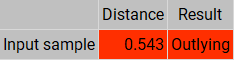
In this case, the distance for this input sample has a value 0.543, which is too high, meaning the sample is classified as outlying.
This is very likely due to an anomaly in the value of the variable turbidity. The mean value of the variable turbidity is 7.66, and in this input sample it is 595.01. Considering the minimum and maximun values of turbidity, the input value strays too far away from a realistic value of this variable.

An example of a stable sample is shown below:

  INPUTS OUTPUTS
Water Temperature 19.0755 19.0594
Turbidity 7.66049 -0.2836
Tranducer Depth 1417.46 1575.0985
Wave Height 148.687 152.2600
Wave Period 3.86446 3.9238
Battery Life 11.075 11.0102

This input sample has a much lower distance than the input sample above this one with a value of 0.062.

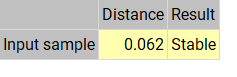
Therefore, this sample is stable.

Conclusions

In conclusion, finding anomalies in beach water using neural networks and auto association techniques can provide valuable insights to ensure the safety and well-being of beachgoers.

This search for an anomaly in the state of the beach can be used for hazard prevention. By utilizing historical data and identifying patterns in environmental factors, we can improve the accuracy of water quality forecasts, allowing for better-informed decisions by beach managers and the public.

Related post