This example aims to build a machine learning model to assess bankruptcy risk based on qualitative parameters provided by experts.
In general, Risk assessment i involves identifying hazards and risk factors that could potentially harm a business, including the possibility of bankruptcy. Therefore, understanding these factors is essential for proactive financial management.
More specifically, bankruptcy is a legal proceeding that occurs when a person or business becomes unable to repay outstanding debts. Consequently, early detection of financial distress can help organizations implement corrective strategies before reaching that stage.
Contents
- Application type.
- Data set.
- Neural network.
- Training strategy.
- Model selection.
- Testing analysis.
- Model deployment.
This example is solved with Neural Designer. In order to follow this example step by step, you can use the free trial.
1. Application type
This is a classification project, since the target variable is binary: bankruptcy or non-bankruptcy. Therefore, the model must distinguish between two possible outcomes.
In this context, the goal is to estimate the probability that a business will go bankrupt based on various qualitative and financial features. As a result, the model provides a risk score that supports early decision-making and preventive action.
2. Data set
The data set contains information to create our model. We need to configure three things:
- Data source.
- Variables.
- Instances.
The data file used for this example is bankruptcy-prevention.csv, which contains 7 features about 250 companies.
The data set includes the following variables:
- industrial_risk: 0=low risk, 0.5=medium risk, 1=high risk.
- management_risk: 0=low risk, 0.5=medium risk, 1=high risk.
- financial_flexibility: 0=low flexibility, 0.5=medium flexibility, 1=high flexibility.
- credibility: 0=low credibility, 0.5=medium credibility, 1=high credibility.
- competitiveness: 0=low competitiveness, 0.5=medium competitiveness, 1=high competitiveness.
- operating_risk: 0=low risk, 0.5=medium risk, 1=high risk.
- class: bankruptcy, non-bankruptcy (target variable).
On the other hand, the instances are divided randomly into training, selection, and testing subsets, containing 60%, 20%, and 20% of the instances, respectively.
Our target variable is class. We can calculate the data distributions and plot a pie chart with the percentage of instances for each class.
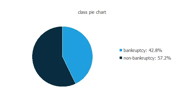
As we can see, the target variable is exceptionally well-balanced. Indeed, 42.8% are positive samples and 57.8% are negative samples.
The inputs-targets correlations might indicate which factors have the greatest influence on going into bankruptcy.
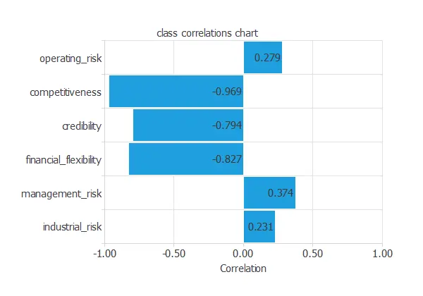
In this example, the variables that correlate the most with the target variable negatively correlate. Competitiveness is the variable with the highest correlation.
3. Neural network
The next step is to set the neural network parameters. For classification problems, it is composed of:
- Scaling layer.
- Perceptron layers.
- Probabilistic layer.
The mean and standard deviation scaling method has been set for the scaling layer.
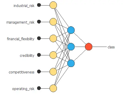
We set one perceptron layer with 3 neurons with the logistic activation function. Since the target variable is binary, this layer has six inputs and only one output.
The neural network for this example can be represented with the following diagram:
4. Training strategy
The fourth step is to set the training strategy defining what the neural network will learn. A general training strategy for classification is composed of two terms:
- A loss index.
- An optimization algorithm.
The loss index chosen for this problem is the normalized squared error between the outputs from the neural network and the targets in the data set with L1 regularization.
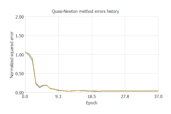
The selected optimization algorithm is the Quasi-Newton method.
The following chart shows how training and selection errors develop with the epochs during training. The final values are training error = 0.0357 NSE and selection error = 0.0285 NSE.
5. Model selection
The objective of model selection is to improve the neural network’s generalization capabilities or, in other words, to reduce the selection error.
Since the selection error we have achieved is minimal (0.0285 NSE), there is no need to apply an order selection or an input selection algorithm.
6. Testing analysis
The objective of the testing analysis is to validate the generalization performance of the trained neural network.
To validate a classification technique, we need to compare the values provided by this technique to the observed values. We can use the ROC curve as it is the standard testing method for binary classification projects.
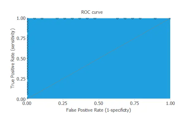
The AUC value for this example is 1.
The following table contains the elements of the confusion matrix. This matrix contains the variable class’s true positives, false positives, false negatives, and true negatives.
| Predicted positive | Predicted negative | |
|---|---|---|
| Real positive | 20 (40%) | 0 (0%) |
| Real negative | 0 (0%) | 30 (60%) |
The total number of testing samples is 50, all correctly classified.
We can also perform the cumulative gain analysis, a visual aid that shows the advantage of using a predictive model instead of randomness.
It consists of three lines. The baseline represents the results that would be obtained without using a model. The positive cumulative gain shows in the y-axis the percentage of positive instances found against the population represented in the x-axis.
Similarly, the negative cumulative gain shows the percentage of the negative instances found against the population percentage.
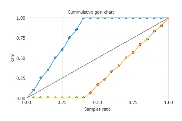
In this case, by using the model, we see that by analyzing 40% of the businesses with a higher probability of going bankrupt, we would reach 100% of the companies that will go bankrupt.
7. Model deployment
In the model deployment phase, we use the neural network to predict the risk of a company.
Mathematical expression
The mathematical expression represented by the predictive model is listed next:
scaled_industrial_risk = (industrial_risk-0.5180000067)/0.4115259945;
scaled_management_risk = (management_risk-0.6140000224)/0.4107050002;
scaled_financial_flexibility = (financial_flexibility-0.3759999871)/0.4015829861;
scaled_credibility = (credibility-0.4699999988)/0.415681988;
scaled_competitiveness = (competitiveness-0.476000011)/0.440681994;
scaled_operating_risk = (operating_risk-0.5699999928)/0.4345749915;

perceptron_layer_1_output_00 = logistic( 0.0068644 + (scaled_industrial_risk*0.00202216) + (scaled_management_risk*-0.0209541) + (scaled_financial_flexibility*0.410356) + (scaled_credibility*0.231337) + (scaled_competitiveness*1.40435) + (scaled_operating_risk*-0.00677014) );
perceptron_layer_1_output_11 = logistic( -0.000410683 + (scaled_industrial_risk*-0.00335452) + (scaled_management_risk*0.00233676) + (scaled_financial_flexibility*0.00435821) + (scaled_credibility*-1.38581e-06) + (scaled_competitiveness*0.00713994) + (scaled_operating_risk*-0.000435457) );
perceptron_layer_1_output_22 = logistic( 0.198992 + (scaled_industrial_risk*0.00149979) + (scaled_management_risk*-0.0878777) + (scaled_financial_flexibility*0.721492) + (scaled_credibility*0.569166) + (scaled_competitiveness*2.23102) + (scaled_operating_risk*-0.0712571) );

probabilistic_layer_combinations_0 = 2.77521 -2.3135*perceptron_layer_1_output_0 +0.00396173*perceptron_layer_1_output_1 -4.69263*perceptron_layer_1_output_2

class = 1.0/(1.0 + exp(-probabilistic_layer_combinations_0);
This formula can also be exported to the software tool the company requires.
References
- The data for this problem has been taken from the Machine Learning UCI Repository.