Introduction
Accurate differentiation between acute lymphoblastic leukemia (ALL) and acute myeloid leukemia (AML) is critical, since treatment approaches and outcomes vary significantly.
Although gene expression data can support this diagnosis, classification is challenging because of the large number of genes and subtle expression differences.
In this study, we trained a neural network using gene expression profiles from 7,129 genes across 72 patients, applying feature selection to identify the most informative markers.
This machine learning approach demonstrates strong potential to assist physicians in leukemia diagnosis and treatment planning.
Healthcare professionals can test the methodology with Neural Designer.
Contents
The following index outlines the steps for performing the analysis.
1. Model type
Problem type: Binary classification (acute lymphoblastic leukemia [ALL] vs. acute myeloid leukemia [AML])
Goal: Model the probability of a patient having AML based on gene expression data obtained from microarray analysis to support clinical decision-making
2. Data set
Data source
The leukemiamicroarray.csv dataset includes 7129 genes and 72 patients, with ALL and AML case distributions.
Variables
The following list summarizes the variables’ information:
Genetic expression
- Gene 1 – Gene 7129 (0–1): Normalized gene expression levels obtained from microarray analysis, where values near 0 indicate low expression and values near 1 indicate high expression.
Some genes show higher correlation with leukemia type:
Gene 4847 – Perfectly correlated with the target variable.
Gene 2288 – Perfectly correlated with the target variable.
Other genes – Varying degrees of correlation, potentially contributing to classification.
Target variable
diagnose (ALL or AML) – Acute lymphoblastic leukemia (ALL) or acute myeloid leukemia (AML).
Variables distributions
We can examine variable distributions; the figure shows a pie chart of total cases, distinguishing AML and AML instances.
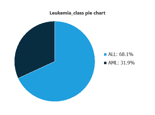
As depicted in the image, ALL cases represent 31.95% of the samples, while AML cases represent approximately 68.06%.
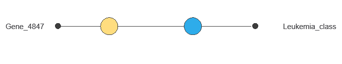
Inputs-targets correlations
The inputs-targets correlations indicate which factors most influence whether a patient has AML or AML and, therefore, are more relevant to our analysis.
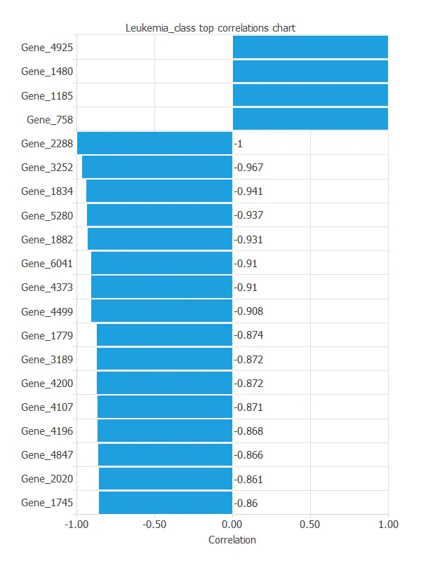
As we can see in the previous figure, some genes have a high correlation with the diagnosis. The genes 4847 and 2288 perfectly correlate with the target variable.
This correlation means that these genes greatly impact the target variable.
To do that, their values must be logistically separable. A certain probability is attached to the random logistical separability of a column with 72 values. It obeys the formula:
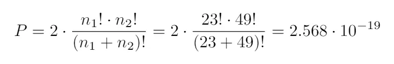
n1 and n2 are the total number of values of AML and ALL, respectively.
This would mean that, for a dataset similar to ours, but with its values set randomly, there may be 1.831·10-15 of the variables that are very correlated only by chance and not by actual correlation. In this case, that number is very small and doesn’t affect our conclusions.
3. Neural network
The neural network is an artificial intelligence model designed to recognize patterns in clinical and genetic data.
It processes the data through scaling and probabilistic layers to calculate the probability that a patient has leukemia.
This probability provides healthcare professionals with an objective measure to guide further tests or early interventions, effectively distinguishing between patients with ALL and AML.
The network itself is not shown due to the large number of input variables.
4. Training strategy
Training a neural network for leukemia classification involves a loss function and optimization algorithm to learn while avoiding overfitting.
Given the large number of variables, the model has not yet been trained; once carefully selected and trained, it will accurately distinguish ALL from AML, supporting clinical decisions.
5. Model selection
The objective of model selection is to find the network architecture with the best generalization properties, which minimizes the error on the selected instances of the data set.
Given that the selection error we have achieved so far is minimal at 0.233, we don’t need to apply order selection or input selection here.
The final training and selection errors are training error = 0.039 WSE and selection error = 0.233 WSE, respectively.
6. Testing analysis
The objective of the testing analysis is to validate the generalization performance of the trained neural network.
ROC curve
The ROC curve is a standard tool to evaluate a classification model, showing how well it distinguishes between two classes by comparing predicted results with actual outcomes, such as patients with ALL or AML.
A random classifier scores 0.5, while a perfect classifier scores 1.
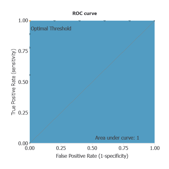
The AUC is 1, showing that the model performs exceptionally well at distinguishing between patients with ALL and AML.
Confusion matrix
The confusion matrix shows the model’s performance by comparing predicted and actual diagnoses. It includes:
True positives: patients correctly identified as having leukemia
False positives: patients incorrectly identified as having leukemia
False negatives: patients with leukemia incorrectly identified as not having it
True negatives: patients correctly identified as not having leukemia
For a decision threshold of 0.5, the confusion matrix was:
| Predicted positive | Predicted negative | |
|---|---|---|
| Real positive | 5 | 0 |
| Real negative | 0 | 9 |
In this case, 100% of cases were correctly classified and 0% were misclassified.
Binary classification
The performance of this binary classification model is summarized with standard measures.
Accuracy: 100% of patients were correctly classified.
Error rate: 0% of cases were misclassified.
Sensitivity: 100% of patients with leukemia were correctly identified.
Specificity: 100% of patients without leukemia were correctly identified.
These measures indicate that the model is highly effective at distinguishing between patients with ALL and AML.
7. Model deployment
Once validated, the neural network can be deployed to predict ALL or AML from new patient gene expression data, providing reliable diagnostic support.
Although the network cannot be practically visualized due to the large number of genes, it can be automatically exported from Neural Designer for use on new datasets.
Conclusions
The leukemia diagnosis model, developed from gene expression data, achieved perfect performance (AUC = 1, accuracy = 100%), accurately distinguishing ALL from AML.
Specific gene markers, such as 4847 and 2288, were strongly associated with leukemia type, aligning with current medical knowledge.
This machine learning model can support early and precise classification, complementing traditional diagnostics and guiding treatment decisions.
References
- Golub,T.R., Slonim,D.K., Tamayo,P., “Molecular Classification of Cancer: Class Discovery and Class Prediction by Gene Expression Monitoring”, Science, Vol. 286, pp. 531-537 (1998).
The development of this application has been funded by the NEMHESYS – NGS Establishment in Multidisciplinary Healthcare Education System project.