This example builds a machine learning model to classify size measurements for adult foraging penguins near Palmer Station, Antarctica.
We used data on 11 variables obtained during penguin sampling in Antarctica.
This data is obtained from the palmerpenguins package.
Contents
1. Application type
The predicted variable can have three values corresponding to a penguin species: Adelie, Gentoo, and Chinstrap. Therefore, this is a multiple classification project.
The goal of this example is to model the probability of each sample belonging to a penguin species.
2. Data set
Data source
The penguin_dataset.csv file contains the data for this example.
Target variables have three values in our classification model: Adelie (0), Gentoo (1), and Chinstrap (2).
The number of rows (instances) in the data set is 334, and the number of variables (columns) is 11.
Variables
The following list summarizes the variables’ information:
- clutch_completion: a character string denoting if the study nest was observed with a full clutch, i.e., 2 eggs.
- date_egg: a date denoting the date the study nest was observed with 1 egg (sampled).
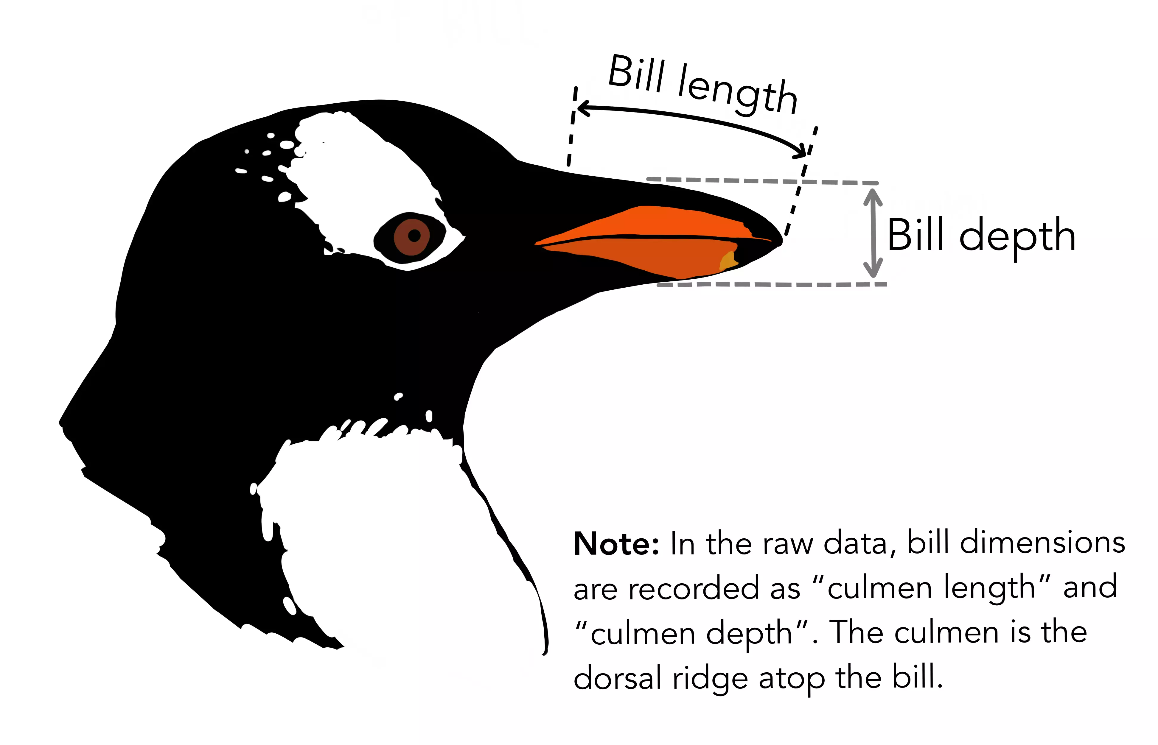
- culmen_length_mm: a number denoting the length of the dorsal ridge of a bird’s bill (millimeters).
- culmen_depth_mm: a number denoting the depth of the dorsal ridge of a bird’s bill (millimeters).
- flipper_length_mm: an integer denoting the length of the penguin’s flipper (millimeters).
- body_mass_g: an integer denoting the penguin’s body mass (grams).
- sex: a factor denoting penguin sex (female, male).
- delta_15_N: a number denoting the measure of the ratio of stable isotopes 15N:14N.
- delta_13_C: a number denoting the measure of the ratio of stable isotopes 13C:12C.
The number of input variables, or attributes for each sample, is 9.
The number of target variables is 1, species (adelie, gentoo, and chinstrap).
Instances
Each row contains the input and target variables of a different instance.
Variables distributions
Also, we can calculate the distributions of all variables. The following pie chart shows the number of species we have.
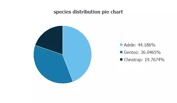
The image shows the proportion of each penguin species: Adelie (44.18%), Gentoo (36,04%), and Chinstrap (19.76%).
Inputs-targets correlations
The input-target correlations might indicate which factors most differentiate between penguins and, therefore, be more relevant to our analysis.
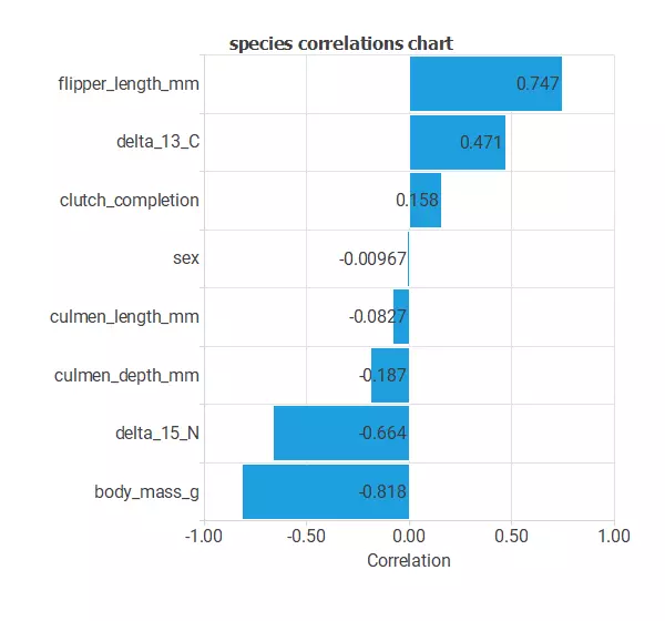
Here, the most correlated variables with penguin species are date_egg, culmen_depth_mm, delta_13_C, and delta_15_N.
3. Neural network
The next step is to set a neural network as the classification function. Usually, the neural network is composed of:
Scaling layer
The scaling layer contains the inputs scaled from the data file and the method used for scaling. Here, the method selected is the minimum-maximum. As we use ten input variables, the scaling layer has ten inputs.
Dense layer
The dense layer applies the Softmax activation to interpret outputs as class probabilities.
It takes ten inputs and produces three outputs.
Each output gives the probability of a sample belonging to a class.
Neural network graph
The following figure represents the neural network:
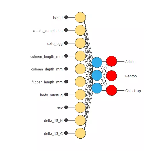
The network takes ten inputs and produces three outputs, which represent the probability of a penguin belonging to a given class.
4. Training strategy
The fourth step is to set the training strategy, which is composed of two terms:
- A loss index.
- An optimization algorithm.
Loss index
The aim is to find a neural network that fits the data set (error term) and does not oscillate (regularization term).
The loss index is the normalized squared error with L2 regularization, the default loss index for classification applications.
Optimization algorithm
The optimization algorithm we use is the quasi-Newton method, the standard optimization algorithm for this type of problem.
Training
The following image shows how the error decreases with the iterations during the training process.
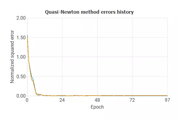
The curves have converged, as we can see in the previous image.
The final errors are 0.004 for training and 0.005 for validation.
However, the selection error is a bit higher than the training error.
6. Testing analysis
The objective of the testing analysis is to validate the generalization properties of the trained neural network.
The method to validate the performance of our model is to compare the predicted values to the real values, using a confusion matrix.
Confusion matrix
The rows represent the real classes in the confusion matrix, and the columns are the predicted classes for the testing data.
The following table contains the values of the confusion matrix.
| Predicted Adelie | Predicted Gentoo | Predicted Chinstrap | |
|---|---|---|---|
| Real Adelie | 22 (32.353%) | 0 | 1 (1.471%) |
| Real Gentoo | 0 | 31 (45.588%) | 1 (1.471%) |
| Real Chinstrap | 0 | 0 | 13 (19.118%) |
As we can see, we can classify 66 (97.1%) of the samples, while we fail to do so for 2 (2.9%) samples
7. Model deployment
Once we have tested the neural network’s performance, we can save it for the future using the model deployment mode.
References
- Artwork by @allison_horst
- This data is obtained from the palmerpenguins package
- Gorman KB, Williams TD, Fraser WR (2014). Ecological sexual dimorphism and environmental variability within a community of Antarctic penguins (genus Pygoscelis). PLoS ONE 9(3):e90081.
- GitHub: Palmerpenguins