In this example, we will build a machine learning model to inspect milk quality by seven observable milk variables.
Milk can be classified in terms of its quality into three groups: low quality, medium quality, and high quality.
The central goal is to design a model that accurately classifies new milk samples. In other words, one that exhibits good generalization.
This example is solved with Neural Designer. To follow it step by step, you can use the free trial.
Contents
1. Application type
This is a classification project. Indeed, the variable to be predicted is categorical (low, medium, and high).
The objective is to model the quality of the milk by knowing its characteristics and thus be able to make future predictions.
2. Data set
The first step is to prepare the dataset, which is the source of information for the classification model.
For that, we need to configure the following concepts:
- Data source.
- Variables.
- Instances.
Data source
The data source for this example is the CSV file milk.csv.
The number of columns is 8, and the number of rows is 1060.
Variables
The variables are:
Numerical variables
- pH – Milk pH, ranging from 3 to 9.5.
- temperature – Milk temperature, ranging from 34 °C to 90 °C.
- colour – Milk color, with values between 240 and 255.
Binary variables
- taste – 1 = good, 0 = bad.
- odor – 1 = good, 0 = bad.
- fat – 1 = good, 0 = bad.
- turbidity – 1 = good, 0 = bad.
Target variable
grade – Milk quality class: low_quality, medium_quality, or high_quality.
All variables in the study are inputs, except “grade”, which is the output that we want to extract from this machine learning study.
Note that “grade” is categorical and can take the values low_quality, medium_quality, and high_quality.
Instances
The instances are randomly split into 60.2% training (637 samples), 19.9% validation (211 samples), and 19.9% testing (211 samples).
Distributions
The following figure is the pie chart for the variable milk quality class, and it shows its distribution.
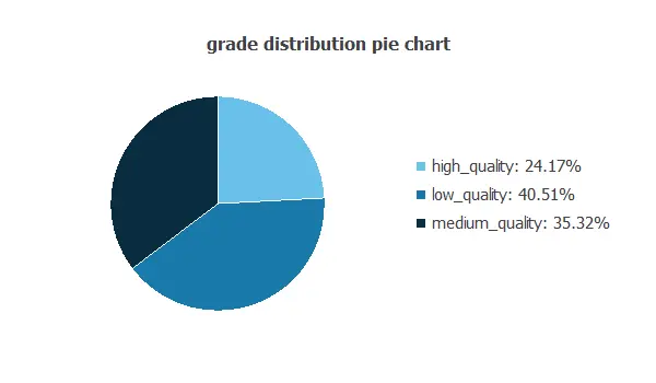
The milk dataset has 429 low-quality, 374 medium-quality, and 256 high-quality instances.
This shows an imbalanced target, with low quality making up 40.5% of the samples and high quality only 24.2%.
3. Neural network
The second step is to choose a neural network.
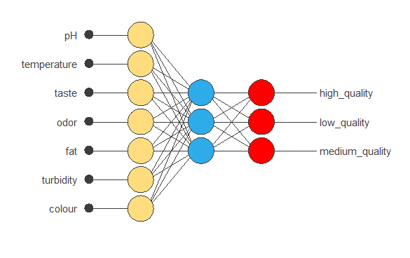
The neural network must have seven inputs since the data set has seven input variables.
The neural network has three outputs because we have three different “grades”: low_quality, medium_quality, and high_quality.
In classification problems, it typically consists of:
- A scaling layer.
- Two dense layers.
Scaling layer
The scaling layer normalizes the input values. As our inputs have different distributions, they are scaled with different methods:
- The variables pH, temperature, and colour are scaled with the mean and standard deviation scaling method.
- The variables taste, odor, fat, and turbidity are scaled with the minimum and maximum scaling method.
Dense layers
In this case, as the first guest, we only use one perceptron layer. This layer contains seven inputs, three neurons, and three outputs. For this example, the perceptron layer is a hyperbolic tangent activation function.
The probabilistic layer allows for interpreting the outputs as probabilities. In this regard, all outputs are between 0 and 1, and their sum is 1. The softmax probabilistic activation is used here.
The following figure is a graphical representation of this classification neural network:
4. Training strategy
The next step is to set the training strategy, which comprises:
- Loss index.
- Optimization algorithm.
Loss index
The loss index chosen for this application is the normalized squared error with L2 regularization.
The error term fits the neural network to the training instances of the data set.
The regularization term makes the model more stable and improves generalization.
Optimization algorithm
The optimization algorithm searches for the neural network parameters that minimize the loss index.
The quasi-Newton method is chosen here.
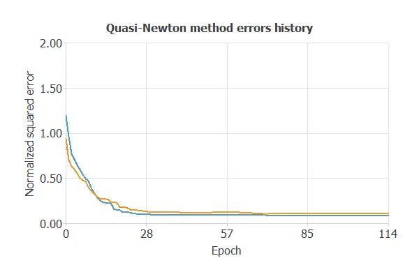
The following chart shows how the training (blue) and selection (orange) errors decrease with the epochs during training.

The final values are training error = 0.252 NSE (blue) and selection error = 0.277 NSE (orange).
5. Model selection
It is essential to have low selection error in our model, allowing us to generalize well to the new data rather than simply memorizing the training data.
The objective of model selection is to find the network architecture with the best generalization properties. That is, the method that minimizes the error on the selected instances of the data set.
We aim to develop a neural network with a selection error of less than 0.277 NSE, the current best value we have achieved.
Neuron selection
Order selection algorithms train several network architectures with a different number of neurons and select the one with the smallest selection error.
The incremental order method starts with a small number of neurons and increases the complexity at each iteration. The following chart shows the training error (blue) and the selection error (yellow) as a function of the number of neurons.
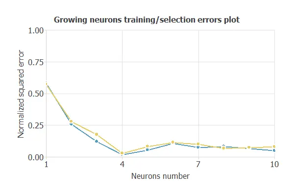
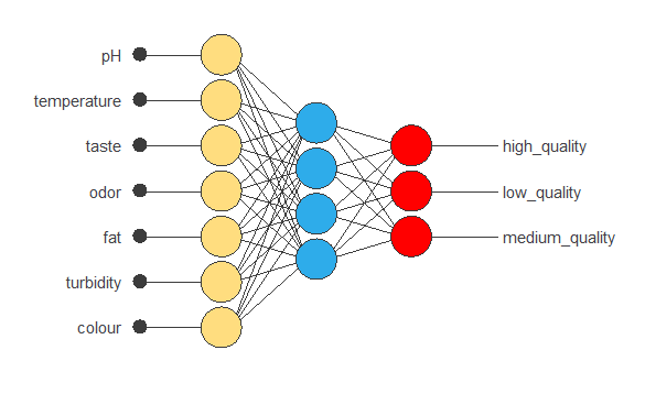
As we can see, the number of neurons that yield the minimum error is four. Therefore, we select the neural network with four neurons in the hidden layer.
The following chart shows the new neural network architecture.
The following chart shows how the training and selection errors decrease with the epochs during training in the new neural network. The final values are training error = 0.0877 NSE (blue) and selection error = 0.107 NSE (orange).
With the new architecture of the neural network, we achieve around 50% less selection error.
6. Testing analysis
The purpose of the testing analysis is to validate the generalization performance of the model.
Here, we compare the neural network outputs to the corresponding targets in the testing instances of the data set.
Confusion matrix
In the confusion matrix, the rows represent the targets (or real values) and the columns the corresponding outputs (or predictive values).
| Predicted low_quality | Predicted medium_quality | Predicted high_quality | Total | |
|---|---|---|---|---|
| Real low_quality | 49 (23.2%) | 0 | 4 (1.9%) | 53 (23.7%) |
| Real medium_quality | 1 (0.5%) | 92 (43.6%) | 0 | 93 (43.6%) |
| Real high_quality | 0 | 0 | 65 (30.8%) | 65 (32.7%) |
| Total | 50 (23.7%) | 92 (43.6%) | 69 (32.7%) | 211 (100%) |
The number of correctly classified samples is 206, and the number of misclassified samples is 5.
Multiple classification metrics
The confusion matrix allows us to calculate the model’s accuracy and error:
- Classification accuracy: 97.6%.
- Error rate: 2.4%.
7. Model deployment
The neural network is now ready to predict outputs for inputs that it has never seen. This process is called model deployment.
Outputs
To classify a sample of milk, we calculate the neural network outputs.
For instance, consider a sample with the following features:
- ph: 6.63
- temperature: 39.2
- taste: 0
- odor: 1
- fat: 1
- turbidity: 1
The neural network outputs for these features are:
- high_quality: 91.2%
- medium_quality: 8.73%
- low_quality: 0.07%
For this particular case, the neural network would classify the sample of milk as being of high quality since it has the highest probability.
We can implement this expression in any programming language to obtain the output for our input.
References
- Kaggle. Machine Learning and Data Science Community: Milk Dataset.