This example demonstrates how machine learning can predict wine preferences to support oenologists in enhancing wine quality.
The model complements tasting evaluations with objective data from laboratory tests.
It can also help producers and marketers understand consumer preferences in niche markets.
The variables come solely from physicochemical analyses, not from grape type, brand, or price.
The model outputs a quality score ranging from 0 to 10.
This application is developed using Neural Designer, a machine learning platform that you can try step by step with our free trial.
Contents
1. Application type
This is an approximation project since the variable to be predicted is continuous (wine quality).
The primary objective is to model the quality of a wine as a function of its characteristics.
2. Data set
The data file wine_quality.csv contains a total of 1599 rows and 12 columns.
Variables
The data set contains the following variables:
- fixed_acidity – Non-volatile acids in wine (e.g., tartaric acid).
- volatile_acidity – Volatile acids that can affect aroma (e.g., acetic acid).
- citric_acid – Citric acid content, which can add freshness.
- residual_sugar – Sugar remaining after fermentation.
- chlorides – Salt content (g/L of sodium chloride).
- free_sulfur_dioxide – Free SO₂, prevents microbial growth.
- total_sulfur_dioxide – Total SO₂ (bound + free).
- density – Density of the wine (g/cm³).
- pH – Measure of acidity (scale of 0–14).
- sulfates – Sulfate content, contributes to SO₂ levels.
- alcohol – Alcohol percentage by volume.
Instances
On the other hand, the instances are randomly divided into training (60%), selection (20%), and testing (20%) subsets.
Distributions
Once the dataset page is edited, we run several related tasks to verify the quality of the provided information.
The following figure illustrates the distribution of the quality variable.
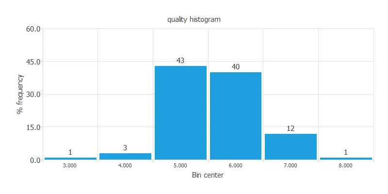
The target variable is unbalanced, with most scores clustered around 5 and 6 and very few near 0 or 10, which can degrade model performance.
Input-target correlations
The following chart illustrates the correlations between the physicochemical characteristics and the quality.
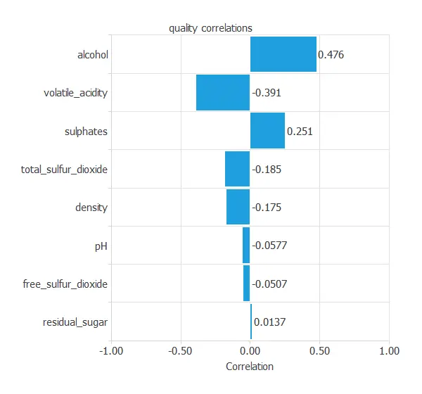
As you can see, alcohol has the highest positive correlation with quality, and volatile acidity has the highest negative correlation.
3. Neural network
The second step is to set up a neural network that learns the relationship between the wine’s laboratory measurements and its quality score.
The network has ten input variables (the wine’s chemical properties) and one output (the predicted quality).
Scaling layer
The scaling layer normalizes the input data so that all variables (such as acidity, alcohol, or pH) are comparable.
Hidden dense layer
The first dense layer, or hidden layer, consists of three neurons that combine the ten input variables to capture complex patterns, much like an oenologist evaluating acidity, aroma, and body together.
Output dense layer
The second dense layer, or output layer, has one neuron that produces the final predicted quality score, just as the oenologist gives an overall judgment of the wine.
Unscaling layer
Next, the unscaling layer unnormalizes the output, so the prediction is expressed in the same quality range as the data.
Bounding layer
Finally, the bounding layer ensures that the predictions fall between 1 and 10, which aligns with the way wine quality is evaluated.
Neural network graph
You can represent the neural network for this example in the following diagram:
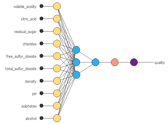
In total, the network contains 37 parameters, which are adjusted during training to provide accurate predictions of wine quality.
4. Training strategy
The next step is to select an appropriate training strategy that defines what the neural network will learn. A general training strategy for approximation consists of two components:
- A loss index.
- An optimization algorithm.
Loss index
The loss index chosen for this problem is the normalized squared error between the neural network’s outputs and the dataset’s targets. On the other hand, we apply L2 regularization with a weak weight in this case.
Optimization algorithm
The selected optimization algorithm is the quasi-Newton method.
Training
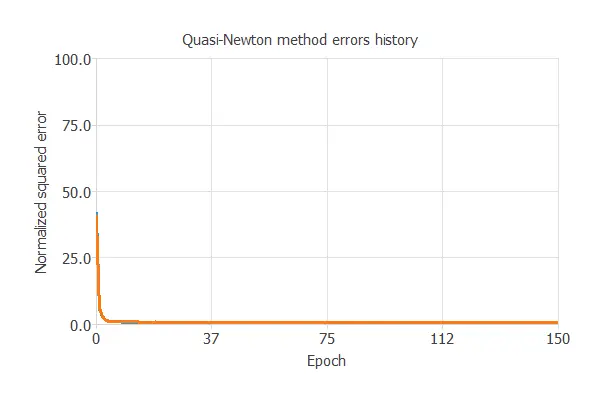
The key training result is the final selection error, which reflects the network’s generalization ability.
In this case, the final selection error is 0.678 NSE.
5. Model selection
The objective of model selection is to find the network architecture with the best generalization properties, which minimizes the error on the selected instances of the data set.
More specifically, we aim to develop a neural network with a selection error of less than 0.678 NSE, which is the current value we have achieved.
Order selection algorithms train several network architectures with different numbers of neurons and select the one with the smallest selection error.
The incremental order method starts with a few neurons and increases the complexity at each iteration. The following chart shows the training error (blue) and the selection error (orange) as a function of the number of neurons.
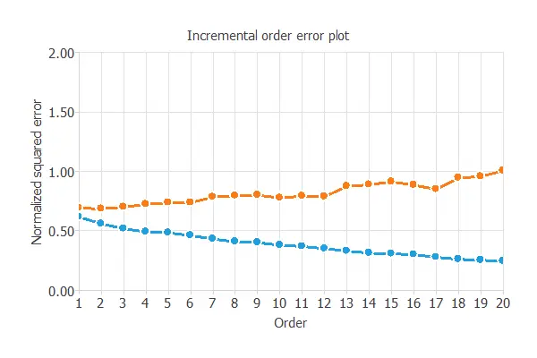
The final selection error achieved is 0.661 for an optimal number of neurons of 1.
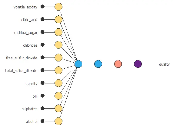
The graph above represents the architecture of the final neural network.
6. Testing analysis
A standard method for testing the prediction capabilities is to compare the neural network outputs with an independent dataset.
Goodnes-of-fit
The linear regression analysis yields three parameters for each output: intercept, slope, and correlation.
The following figure shows the results of this analysis.
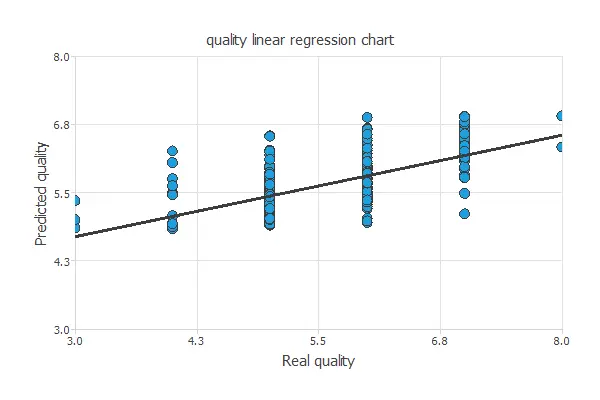
If the correlation equals 1, then there is a perfect correlation between the outputs from the neural network and the targets in the testing subset.
For this case, the correlation has an R-squared value of 0.58, indicating that the model is not performing very well, but still recognizes quality patterns.
As mentioned earlier, the data quality exhibits a significant imbalance, as evident from the preceding graph.
7. Model deployment
After all the steps, we haven’t achieved the best possible model. Nevertheless, it is still better than guessing randomly.
The following listing shows the mathematical expression of the predictive model.
scaled_volatile_acidity = (volatile_acidity-0.527821)/0.17906;
scaled_citric_acid = (citric_acid-0.270976)/0.194801;
scaled_residual_sugar = (residual_sugar-2.53881)/1.40993;
scaled_chlorides = (chlorides-0.0874665)/0.0470653;
scaled_free_sulfur_dioxide = (free_sulfur_dioxide-15.8749)/10.4602;
scaled_total_sulfur_dioxide = (total_sulfur_dioxide-46.4678)/32.8953;
scaled_density = (density-0.996747)/0.00188733;
scaled_pH = (pH-3.31111)/0.154386;
scaled_sulfates = (sulfates-0.658149)/0.169507;
scaled_alcohol = (alcohol-10.423)/1.06567;
y_1_1 = tanh (-0.271612+ (scaled_volatile_acidity*-0.313035)+ (scaled_citric_acid*-0.124956)+ (scaled_residual_sugar*0.00194975)+ (scaled_chlorides*-0.0802881)+ (scaled_free_sulfur_dioxide*0.0392384)+ (scaled_total_sulfur_dioxide*-0.111936)+ (scaled_density*0.0456105)+ (scaled_pH*-0.11043)+ (scaled_sulfates*0.122299)+ (scaled_alcohol*0.361693));
scaled_quality =  (0.159294+ (y_1_1*0.453138));
quality = (0.5*(scaled_quality+1.0)*(8-3)+3);
quality = max(1, quality)
quality = min(10, quality)
You can export the formula below to the software tool the customer requires.