This study aims to classify different raisins using machine learning.
Several traditional methods exist for assessing and determining the raisin type, but they can be time-consuming and tedious.
To solve this problem, we can use machine learning to classify the different types of raisins and thus facilitate the treatment of the raisins.
Contents
- Application type.
- Data set.
- Neural network.
- Training strategy.
- Model selection.
- Testing analysis.
- Model deployment.
This example is solved with Neural Designer. To follow it step by step, you can use the free trial.
1. Application type
We will predict between two types of raisins, so the variable to be predicted is binary (Kecimen or Besni). Therefore, this is a classification project.
The goal is to model the type of raisin based on its features for subsequent use.
2. Data set
The first step is to prepare the data set, which is the source of information for the problem. We need to configure three things here:
- Data source.
- Variables.
- Instances.
Data source
The data file raisin_dataset.csv contains the data for this example. 900 raisins were used, including 450 from both varieties and seven features were extracted. Here, the number of variables (columns) is 8, and the number of instances (rows) is 900.
Variables
The features or variables are the following:
- Area: Gives the number of pixels within the boundaries of the raisin.
- Perimeter: It measures the environment by calculating the distance between the boundaries of the raisin and the pixels around it.
- MajorAxisLenght: Specifies the length of the major axis, denoting the longest line drawable on the raisin.
- MinorAxisLenght: Indicates the length of the small axis, representing the shortest line drawable on the raisin.
- Eccentricity: It measures the ellipse’s eccentricity, which has the same moments as raisins.
- ConvexArea: Gives the number of pixels of the smallest convex shell of the region formed by the raisin.
- Extent: It gives the ratio of the region the raisin forms to the total pixels in the bounding box.
- Class: Kecimen and Besni raisin.
All variables in the study are inputs, except ‘Class’, the output we want to extract for this machine learning study. Note that ‘Class’ is binary and only takes Kecimen and Besni’s values.
Instances
The instances are divided into training, selection, and testing subsets. They account for 540 (60%), 180 (20%), and 180 (20%) of the original instances, respectively, distributed randomly across the dataset.
We can perform a few related analytics once the data set has been set. First, we check the provided information and ensure that the data is of good quality.
Variables distributions
The data distributions tell us the percentages of Kecimen and Besni raisins.
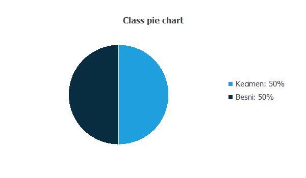
This data set has the same number of samples of both categories (Kecimen and Besni).
Inputs-targets correlations
The input-target correlations might indicate to us which factors are more influential.
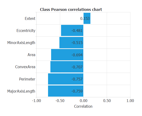
From the above chart, we can see that all the features have a significant influence except the ‘Extent’, compared to the others.
3. Neural network
The second step is to choose a neural network to represent the classification function. Classification problems it consist of:
The scaling layer contains the statistics on the input calculated from the data file and the method for scaling the input variables. Here, the minimum and maximum scaling method is set, but the mean and standard deviation scaling method produces similar results.
We set one perceptron layer, with 3 neurons as a first guess, having the hyperbolic tangent (tanh) as the activation function.
The following figure is a diagram of the neural network used in this example.
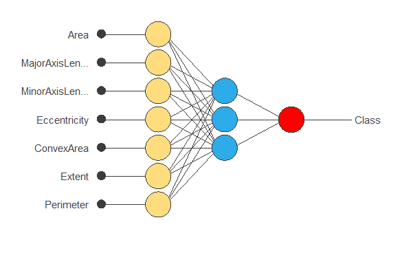
The yellow circles represent scaling neurons, the blue circles perceptron neurons, and the red circles probabilistic neurons. The number of inputs is 7, and the number of outputs is 1.
4. Training strategy
The training strategy is applied to the neural network to obtain the best possible performance. It comprises two components:
- A loss index.
- An optimization algorithm.
The selected loss index is the normalized squared error (NSE) with L2 regularization. In situations with balanced targets, like in this case, the normalized squared error provides valuable assistance.
The error term fits the neural network to the training instances of the data set. The regularization term makes the model more stable and improves generalization, so our model will be more predictive.
The selected optimization algorithm that minimizes the loss index is the quasi-Newton method.
The following chart shows how the training (blue) and selection (orange) errors decrease with the training epochs.
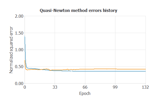
The final training and selection errors are training error = 0.353 NSE (blue) and selection error = 0.419 NSE (orange). The following section will improve the generalization performance by reducing the selection error.
5. Model selection
The objective of model selection is to find the network architecture with the best generalization properties. We want to improve the final selection error obtained before (0.419 NSE).
The best selection error is achieved using a model whose complexity is the most appropriate to produce a better data fit. Order selection algorithms are responsible for finding the optimal number of perceptron neurons in the neural networks.
The following chart shows the error history for different numbers of perceptron neurons. We conclude that for two neurons, the selection error is the minimum.
.webp)
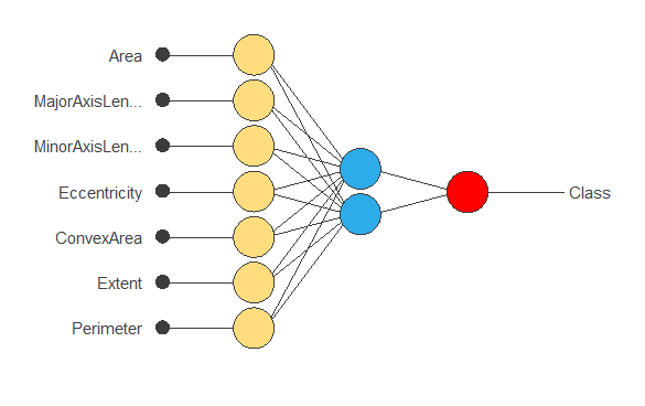
The chart shows that the optimal number of neurons is 2, with selection error = 0.398 NSE.
The following figure shows the final network architecture for this application.
6. Testing analysis
The next step is to perform an exhaustive testing analysis to validate the neural network’s predictive capabilities. The testing compares the values provided by this technique to the observed values.
A good measure of the precision of a binary classification model is the ROC curve. Furthermore, the ROC curve analysis returns the optimal value for the decision threshold = 0.63.
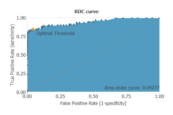
We are interested in the area under the curve (AUC). A perfect classifier would have an AUC=1, and a random one would have an AUC=0.5.
Our model has an AUC of 0.942, which is a good indicator of our model’s performance.
We can also look at the confusion matrix. Next, we show the elements of this matrix for a decision threshold = 0.63.
| Predicted positive | Predicted negative | |
|---|---|---|
| Real positive | 87 (48.3%) | 4 (2.2%) |
| Real negative | 14 (7.8%) | 75 (41.7%) |
From the above confusion matrix, we can calculate the following binary classification tests:
- Classification accuracy: 90% (ratio of correctly classified samples).
- Error rate: 10% (ratio of misclassified samples).
- Sensitivity: 95.6% (percentage of actual positives classified as positive).
- Specificity: 84.26% (percentage of actual negatives classified as negative).
7. Model deployment
Once we have tested the raisin model classification, we can use it to evaluate the probability selection:
For instance, consider a raisin with the following features:
- Area: 80804.1
- MajorAxisLenght: 410.93
- MinorAxisLenght: 224.488
- Eccentricity: 86186.1
- ConvexArea: 86186.1
- Extent: 0.599
- Perimeter: 1005.91
- Class(1=Kecimen): 0.915
The probability of Kecimen for this raisin is: 91.5%.
We can export the mathematical expression of the neural network to any raisin factory to facilitate the work of classification.
This expression is listed below.
scaled_Area = (Area-87804.10156)/38980.39844;
scaled_MajorAxisLength = (MajorAxisLength-430.9299927)/115.9710007;
scaled_MinorAxisLength = (MinorAxisLength-254.4880066)/49.96110153;
scaled_Eccentricity = (Eccentricity-0.7815420032)/0.09026820213;
scaled_ConvexArea = (ConvexArea-91186.10156)/40746.60156;
scaled_Extent = (Extent-0.6995080113)/0.05343849957;
scaled_Perimeter = (Perimeter-1165.910034)/273.6119995;
perceptron_layer_1_output_0 = tanh( 0.625073 + (scaled_Area*0.47795) + (scaled_MajorAxisLength*0.54666) + (scaled_MinorAxisLength*0.222985) + (scaled_Eccentricity*0.277638) + (scaled_ConvexArea*0.506997) + (scaled_Extent*0.77402) + (scaled_Perimeter*1.16189) );
perceptron_layer_1_output_1 = tanh( 0.661286 + (scaled_Area*0.00797501) + (scaled_MajorAxisLength*-0.703279) + (scaled_MinorAxisLength*-0.0445966) + (scaled_Eccentricity*0.069447) + (scaled_ConvexArea*-0.392766) + (scaled_Extent*-0.24135) + (scaled_Perimeter*-1.36504) );
perceptron_layer_1_output_2 = tanh( -0.0796286 + (scaled_Area*1.34031) + (scaled_MajorAxisLength*0.191064) + (scaled_MinorAxisLength*0.612609) + (scaled_Eccentricity*0.207755) + (scaled_ConvexArea*-0.557862) + (scaled_Extent*-0.0264986) + (scaled_Perimeter*-2.60166) );
probabilistic_layer_combinations_0 = -0.90159 +0.58348*perceptron_layer_1_output_0 +1.53865*perceptron_layer_1_output_1 +3.4659*perceptron_layer_1_output_2
Class = 1.0/(1.0 + exp(-probabilistic_layer_combinations_0) );
In conclusion, we have to build a predictive model to determine the kind of raisin.