In this post, we develop a machine learning model to predict forest fires.
Forest fires lead to deforestation, biodiversity loss, air pollution, soil erosion, and ecosystem disruption, causing severe environmental issues.
Contents
1. Application type
This is a classification project since the variable to be predicted is binary (fire or no fire).
The goal is to model the probability of a fire occurring according to the day, month, certain meteorological variables, and a series of indices developed by the FWI system.
2. Data set
The data set comprises a data matrix in which columns represent variables and rows represent instances.
The data file forestfires.csv contains the data needed to create the model.
Here, the number of variables is 9, and the number of instances is 515.
Variables
This data set contains the following variables that contain data measured in the northeast region of Portugal:
Temporal variable
month – Month of observation.
FWY system indices
- FFMC – Fine Fuel Moisture Code.
- DMC – Duff Moisture Code.
- DC – Drought Code.
- ISI – Initial Spread Index.
Weather variables
- temp – Temperature (°C).
- RH – Relative humidity (%).
- wind – Wind speed (km/h).
Target variable
class – Fire occurrence (1 = fire, 0 = not fire).
Instances
Each instance in the dataset represents the fire weather conditions of a specific area and month, including fuel moisture indices, temperature, humidity, wind speed, and whether a fire occurred.
The dataset contains 515 instances, split into 333 for training (80%), 45 for validation (10%), and 45 for testing (10%).
Statistics
We can perform a few related analytics once the data set is set up. First, we check the provided information and ensure that the data is of high quality.
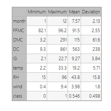
You can calculate data statistics and create a table with the minimum, maximum, mean, and standard deviation for each variable.
The table below shows these values.
Distributions
Also, we can calculate the distributions for all variables. The following figure shows a pie chart with the proportion of fire (positives) and no fire (negatives) following our dataset.
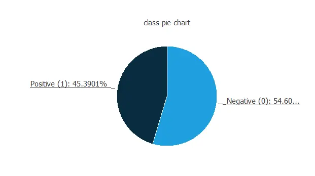
As we can see, the number of fire cases is 45.4% of the samples, and non-fire fire represent approximately 54.6% of the pieces.
Input-target correlations
Finally, the input-target correlations might indicate what factors most influence fires.
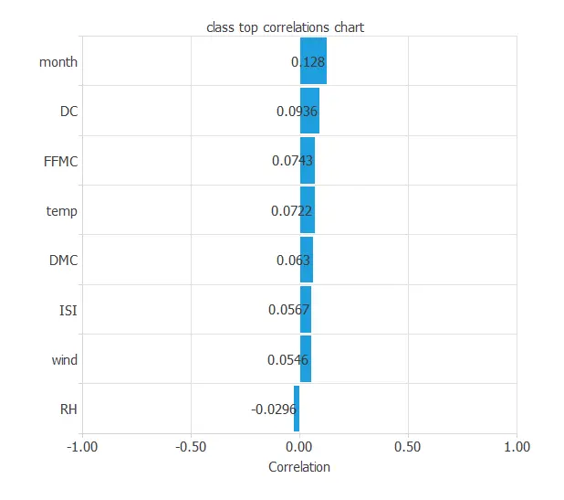
Here, the different variables are a little correlated. Indeed, a forest fire depends on many factors simultaneously.
3. Neural network
The second step is to set a neural network representing the classification function. For this class of applications, the neural network is composed of:
- Scaling layer.
- Perceptron layers.
- Probabilistic layer.
Scaling layer
The scaling layer stores the input statistics from the data file and the chosen scaling method.
In this case, the min–max method is used, though mean–std scaling would give similar results.
Dense layers
The number of perceptron layers is 1. This perceptron layer has 8 inputs and 8 neurons.
Finally, we will set the binary probabilistic method for the probabilistic layer, as we want the predicted target variable to be binary.
Neural network graph
The following picture shows a graph of the neural network for this example.
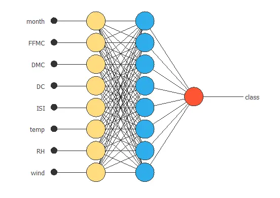
The yellow circles represent scaling neurons, the blue circles perceptron neurons, and the red circles probabilistic neurons. The number of inputs is 8, and the number of outputs is 1.
4. Training strategy
The procedure used to carry out the learning process is called a training strategy. The training strategy is applied to the neural network to obtain the best possible performance. The type of training is determined by how the parameters in the neural network are adjusted.
This process is composed of two terms:
- A loss index.
- An optimization algorithm.
Loss index
The loss index that we use is the weighted squared error with L2 regularization. This is the default loss index for binary classification applications.
The learning problem is finding a neural network that minimizes the loss index. That is a neural network that fits the data set (error term) and does not oscillate (regularization term).
Optimization algorithm
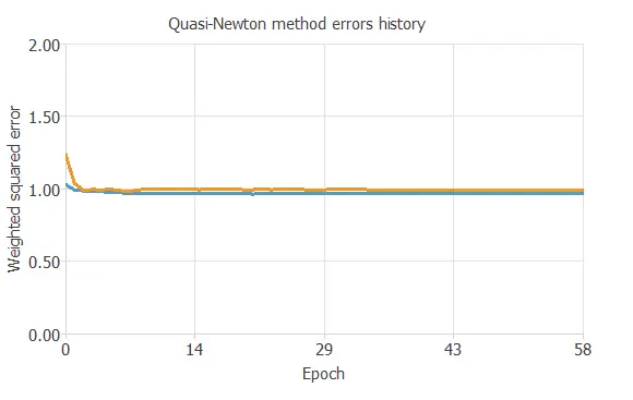
The optimization algorithm that we use is the quasi-Newton method. This is also the standard optimization algorithm for this type of problem.
Training
The following chart shows how errors decrease with the iterations during training.
5. Model selection
The objective of model selection is to find the network architecture with the best generalization properties, which minimizes the error on the selected instances of the data set.
More specifically, we aim to develop a neural network with a selection error of less than 0.933 WSE, the current best value we have achieved.
Order selection algorithms train several network architectures with a different number of neurons and select the one with the smallest selection error.
The incremental order method starts with a few neurons and increases the complexity at each iteration.
6. Testing analysis
The last step is to test the generalization performance of the trained neural network.
The objective of the testing analysis is to validate the generalization performance of the trained neural network. To validate a classification technique, we need to compare the values provided by this technique to the observed values.
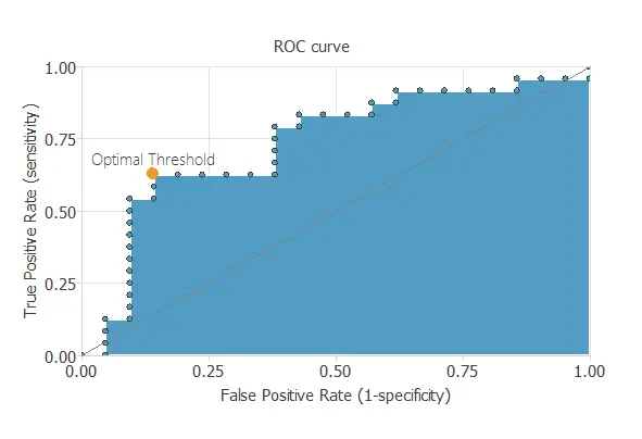
ROC curve
We can use the ROC curve as it is the standard testing method for binary classification projects.
Confusion matrix
In the confusion matrix, the rows represent the target classes, and the columns are the output classes for the testing target data set. The diagonal cells in each table show the number of correctly classified cases, and the off-diagonal cells show the misclassified instances.
The following table shows the confusion matrix elements for this application. The following table contains the elements of the confusion matrix.
| Predicted positive | Predicted negative | |
|---|---|---|
| Real positive | 13 (28.9%) | 8 (18.7%) |
| Real negative | 7 (15.6%) | 17 (37.8%) |
As we can see, the model correctly predicts 30 instances (66.7%) and misclassifies 15 (33.3%).
Binary classification metrics
The following list depicts the binary classification tests for this application:
- Classification accuracy: 66.7% (ratio of correctly classified samples).
- Error rate: 33.3% (ratio of misclassified samples).
- Sensitivity: 61.9% (percentage of actual positives classified as positive).
- Specificity: 70.8% (percentage of actual negatives classified as negative).
7. Model deployment
The neural network is now ready to predict outputs for inputs it has never seen.
Neural network outputs
Below, a specific prediction having determined values for the model’s input variables is shown.
- month: 6 (June)
- FFMC: 75.12
- DMC: 94.26
- DC: 462.3
- ISI: 7.6
- temperature: 15.8 ºC
- RH: 36.0 %
- wind: 3.3 km/h
- Fire probability: 74 %
The model predicts that the previous values correspond to a fire probability of 74%.
Risk map
With the previous algorithm created, we can predict the fire risk and generate a fire risk map.
The following images show an example of such a map:
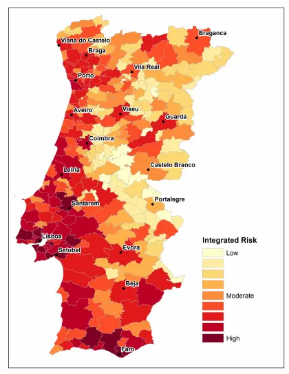
The image above shows the forest fire risk in Portugal.
References
- The data for this problem has been taken from the UCI Machine Learning Repository.
- [Cortez and Morais, 2007] P. Cortez and A. Morais. A Data Mining Approach to Predict Forest Fires using Meteorological Data. In J. Neves, M. F. Santos and J. Machado Eds., New Trends in Artificial Intelligence, Proceedings of the 13th EPIA 2007 – Portuguese Conference on Artificial Intelligence, December, Guimares, Portugal, pp. 512-523, 2007. APPIA, ISBN-13 978-989-95618-0-9. Web Link.
- Portugal fire risk map image Web Link.