Forecasting power demand is crucial for planning and operating electrical systems.
Utilities use short-, medium-, and long-term forecasting, but electricity demand depends on complex meteorological and socio-economic factors, making traditional methods insufficient.
Machine learning offers more advanced ways to capture these dynamics.
In this post, we demonstrate how by building a neural network to predict electricity demand using a real dataset from Kaggle, a leading data science repository.
Contents
1. Data set
A good model for predicting the electricity demand requires analysis of the following types of variables:
- Calendar data: Season, hour, bank holidays, etc.
- Weather data: Temperature, humidity, rainfall, etc.
- Company data: Price of electricity, promotions, marketing campaigns, etc.
- Social data: Economic and political factors that a country is experimenting with.
- Demand data: Historical consumption of electricity.
The data set of our example contains the hourly temperatures and electrical demands for four years. This adds up to more than 70,000 data.
The first column represents the date and time when each instance is measured. The following column is the ambient temperature, and the last column is the electric power demand for that hour of the day.
Time series charts
The time series charts of our dataset are represented here. The first one is the temperature at 23:00 for the final period of our dataset.
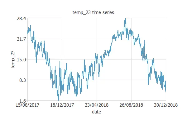
This figure starts in summer with the highest temperatures. Then, it gets the coldest in December and January. We can observe the next peak during August and how the temperature lowers again for winter.
The time-series chart for the demand at 23:00 is represented in the following figure.
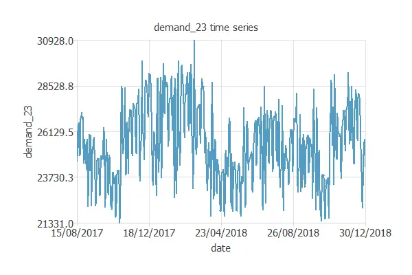
This chart shows that at 23:00, the demand is much more significant in winter.
It is cold, so people usually use more electricity for the heating system. During the summer, there is a smaller peak in the electricity expenditure. In this case, it is used for the air conditioner.
Lags and steps ahead
The data set is transformed into a group of instances where the inputs represent historical data, and the targets represent future information.
The temperature associated with future demand will also be used as an input variable because it can be determined in advance.
In this case, we have set the project configuration to predict the coming day from the data of the previous two days.
For that purpose, the number of input variables will be 125, and the number of target variables will be 24.
Scatter charts
Scatter charts can help us understand how electric power demand depends on the different features.
The first scatter chart represents the relationship between demand and temperature.
This case represents tomorrow’s demand against today’s temperature at the same hour.
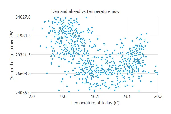
As we can see in the previous picture, the highest demand for tomorrow is at the time of the lowest temperature.
Then, the demand lowers as the temperature reaches a pleasant value (16-20 ºC). It rises again when the temperature is higher.
The following scatter chart shows the current demand against past demands.
We plot tomorrow’s demand against today’s demand at the same hour.
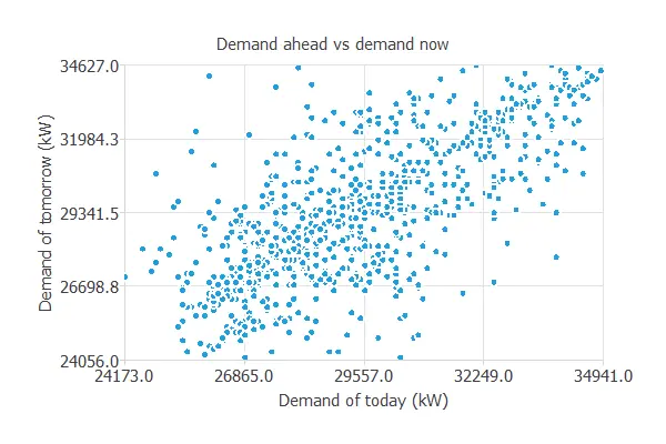
There is a high correlation between these values.
Predictive model
This data is combined in a single predictive model to discover associations between all the above variables.
This will give us a more in-depth understanding of the causes of demand and enable more informed decision-making.
Neural network
Neural networks can anticipate customer responses about energy consumption by considering all relevant factors.
The result is improved forecast accuracy, which means better information for decision-making.
Here is a diagram that depicts the neural network that we will use in this example

Model selection
Order selection algorithms are used to get the optimal number of neurons in a neural network.
In this case, the incremental order method is used.
The following chart shows the loss history for the different subsets during the incremental order selection process. The blue line represents the training loss, and the yellow line symbolizes the selection error.
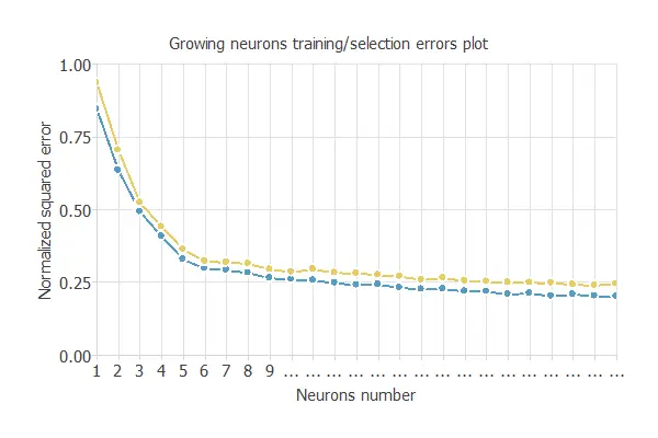
As shown in the previous picture, the optimal order is 24.
Finally, the architecture of this neural network can be written as 125:24:24.
Testing analysis
The objective of the testing analysis is to evaluate the predictive power of the neural network on new data that have not been seen before: the testing instances.
This process will determine if the predictive model is good enough to be moved into the deployment phase.
First, we perform the linear regression analysis between the scaled neural network outputs and the corresponding targets for an independent testing subset.
The following figure represents the linear regression chart of the predicted demand at 1:00.
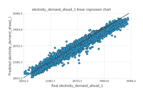
The correlation is very similar to 1. Therefore, the neural network predicts the testing instances well.
Finally, we calculate the error statistics. The mean percentage error obtained using the previous value as the prediction is 5.04%. We have an error of 3.10% using the model, which enables us to make more accurate predictions. Therefore, we can deploy the model.
Model deployment
Once we have tested our predictive model, we can apply it to predict the electric power demand for tomorrow. This process is called model deployment.
The following figure shows the hourly electric power demand prediction for tomorrow in kW, considering the following inputs: yesterday’s, today’s, and tomorrow’s temperatures and yesterday’s and today’s power demands.
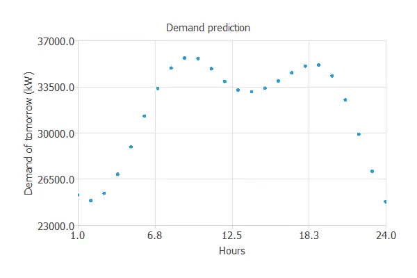
As we can see, the graph looks as expected. Between 5:00 and 8:00, the electricity demand will increase by 10 MW.
This phenomenon matches the beginning of residential, industrial, and service activities.
The second peak occurs around 18:00, primarily because most people return home at this time, leading to an increase in activities such as turning on the heating system.
Conclusions
Machine learning permits us to model and understand very complex systems.
That allows companies to represent the complexity of electricity demand in a previously unachievable way.
More specifically, the objective is to achieve more accurate forecasts for the electricity demand.
Due to predictive analytics, we can predict tomorrow’s electric demand with highly successful results.
For that reason, this will be a significant advance for companies in the energy sector.
The use of machine learning means better information to inform the best course of action.
Therefore, companies that use this technology will have a competitive advantage.
You can use the data science and machine learning platform Neural Designer to build your predictive models in just a few clicks. Download Neural Designer now and try it for free.