Contents

1. Application type.
2. Data set.
3. Neural network.
4. Training strategy.
5. Model selection.
6. Testing analysis.
7. Model deployment.

This example is solved with Neural Designer. To follow it step by step, you can use the free trial.

Volve is an oil field in the Norwegian North Sea near Stavanger. Equinor and partners have published all field data online for research and development. Volve, discovered in 1993, extracted oil and gas between 2008 and 2016. The implementation of water injection sustained pressure, effectively doubling the field’s lifespan beyond its initial expectations.

A lot of data is available for analysis. In this example, we focus on well 5351, which produced more than 40% of the total oil production from the field.

1. Application type

This forecasting project focuses on predicting the value of oil production rates in the coming days using artificial intelligence and machine learning techniques.

The objective is to obtain an accurate prediction based on available data and use these predictions to improve production processes and identify potential problems.

2. Data set

Data source

The volve_field_data.csv file contains 2959 samples, each with 7 input features collected from 2008 to 2016. The dataset undergoes a transformation into a time series, incorporating lagged values and forward steps, serving the purpose of forecasting.

Variables

The following list summarizes the variable’s information:

• down_hole_presure: the pressure of the fluid at the bottom of a wellbore in bars.
• down_hole_temperature: the average temperature of the fluid at the bottom of a wellbore in degrees Celsius.
• production_pipe_pressure: the difference in pressure between two points in the production pipeline in bars.
• choke_size_pct: percentage of choke valve used to control the fluid flow rate in a wellbore.
• well_head_presure: the pressure of the fluid at the top of a wellbore in bars.
• well_head_temperature: the temperature of the fluid at the top of a wellbore in degrees Celsius.
• choke_size_pressure: the pressure difference across a wellbore choke valve.

The target variable oil represents the volume of oil per day in cubic meters.

Instances

The dataset is split into training, validation, and testing subsets, with 60% instances assigned for training, 20% for validation, and 20% for testing by Neural Designer. The user can change these values as desired.

Once the data set has been set, we are ready to perform a few related analytics. With that, we check the provided information and ensure the data is quality.

Variables statistics

We can calculate the data statistics and draw a table with the minimums, maximums, means, and standard deviations of all variables in the data set. The following table displays the values.

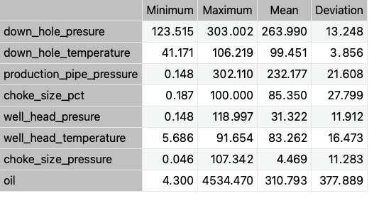
We observed a significant deviation in oil production. The multiple production-related wellbore shutdowns may explain this.

Inputs-targets correlations

Additionally, we can obtain the existing inputs-targets correlations for each variable, which allows us to know the importance of the different influences on oil production.

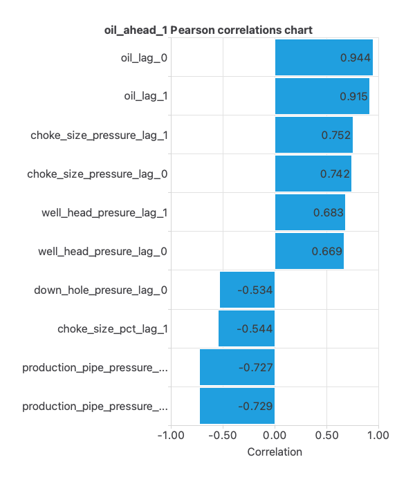
For example, we can see a strong and negative correlation between oil production and pipe_production_pressure, which means that as one increases, the other decreases.

The negative correlation between oil production and pipeline pressure is logical, as a decrease indicates more efficient oil flow and higher production. An increase in pressure signals production issues and lower production.

3. Neural network

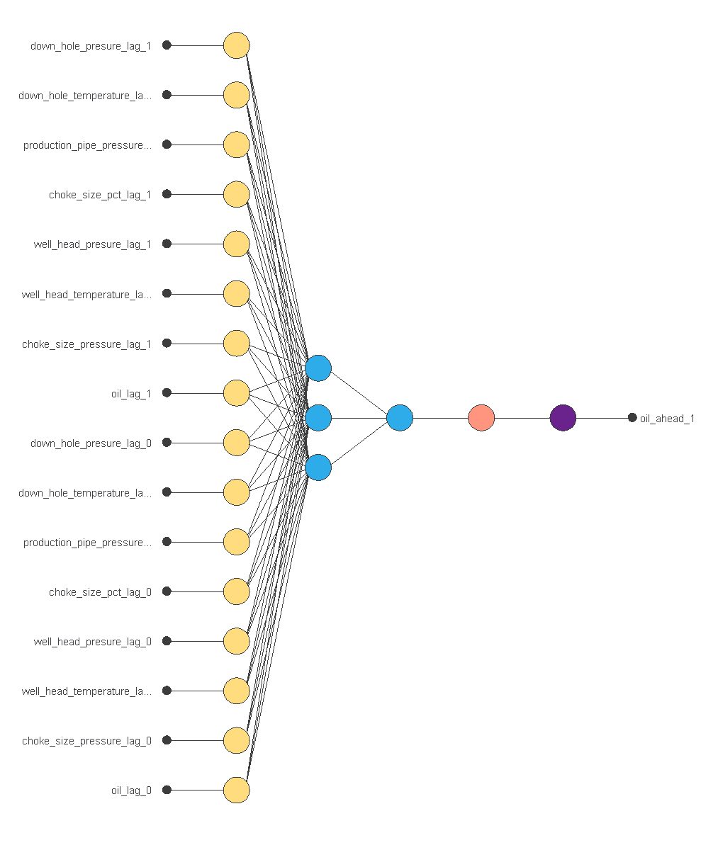
The next step is to set a neural network representing the approximation function. In this class of applications, the neural network comprises:

• Scaling layer.
• Perceptron layer.
• Unscaling layer.
• Bounding layer.

The scaling layer contains the statistics on the inputs calculated from the data file and the method for scaling the input variables. Here the minimum-maximum method has been set. As we use 16 input variables, the scaling layer has 16 inputs.

We use 2 perceptron layers here:

• The first perceptron layer has 16 inputs, 3 neurons, and a hyperbolic tangent activation function
• The second perceptron layer has 3 inputs, 1 neuron, and a linear activation function

The unscaling layer contains the statistics of the output.

The following figure is a graphical representation of this neural network.

4. Training strategy

A training strategy is used to carry out the learning process. Then, we apply the training strategy to the neural network to optimize its performance. How the parameters adjust in the neural network determines the type of training.

We set the weighted squared error with L2 regularization as the loss index.

On the other hand, we use the quasi-Newton method as optimization algorithm.

The following chart shows how the training and selection errors decrease with the quasi-Newton method’s epochs during the training process.

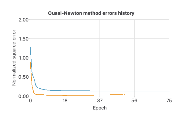
The previous chart shows how the training (blue) and selection (orange) errors decrease with the epochs during the training process. The final values are training error = 0.125 ME and selection error = 0.027 ME. That indicates that the neural network has good generalization capabilities.

5. Model selection

The objective of model selection is to find the network architecture with the best generalization properties, which minimizes the error on the selected instances of the data set.

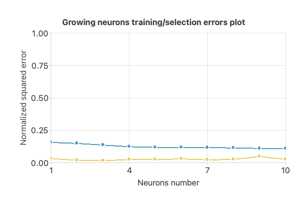
Order selection algorithms train several network architectures with a different number of neurons and select that with the smallest selection error.

The incremental order method starts with a small number of neurons and increases the complexity at each iteration.
The following chart shows the training error (blue) and the selection error (yellow) as a function of the number of neurons.

6. Testing analysis

Once the model is trained, we perform a testing analysis to validate its prediction capacity. We use a subset of data that has not been used before, the testing instances.

To verify the results obtained in this example, the graphs displaying the comparison between the actual oil production values are below.

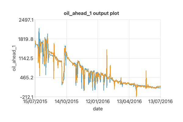
The oil precision graph shows a good match between the prediction and actual results, leading to satisfactory outcomes.

On the other hand, the following table presents the relative error obtained using the previous value as a prediction (base model) and the neural network model.

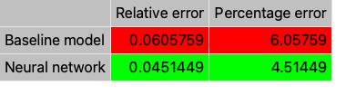
As we can see, this comparison demonstrates the effectiveness of the neural network model versus the baseline prediction technique.

7. Model deployment

The neural network is now ready to predict the activity of new people in the so-called model deployment phase.

The file volve-field-forecasting.py implements the mathematical expression of the neural network in Python. This piece of software can be embedded in any tool to make predictions on new data.

Besides, we can use the mathematical expression of the neural network, which is listed next.

scaled_down_hole_presure_lag_1 = (down_hole_presure_lag_1-252.3179932)/18.92510033;
scaled_down_hole_temperature_lag_1 = (down_hole_temperature_lag_1-101.1409988)/4.748660088;
scaled_production_pipe_pressure_lag_1 = (production_pipe_pressure_lag_1-214.6000061)/26.03879929;
scaled_choke_size_pct_lag_1 = (choke_size_pct_lag_1-78.42089844)/28.24139977;
scaled_well_head_presure_lag_1 = (well_head_presure_lag_1-37.50559998)/16.14410019;
scaled_well_head_temperature_lag_1 = (well_head_temperature_lag_1-83.3812027)/16.26160049;
scaled_choke_size_pressure_lag_1 = (choke_size_pressure_lag_1-9.438480377)/17.18700027;
scaled_oil_lag_1 = (oil_lag_1-898.6339722)/731.4899902;
scaled_down_hole_presure_lag_0 = (down_hole_presure_lag_0-252.2980042)/19.25939941;
scaled_down_hole_temperature_lag_0 = (down_hole_temperature_lag_0-101.0879974)/4.937150002;
scaled_production_pipe_pressure_lag_0 = (production_pipe_pressure_lag_0-214.5690002)/26.19440079;
scaled_choke_size_pct_lag_0 = (choke_size_pct_lag_0-78.34420013)/28.36770058;
scaled_well_head_presure_lag_0 = (well_head_presure_lag_0-37.54339981)/16.26230049;
scaled_well_head_temperature_lag_0 = (well_head_temperature_lag_0-83.2582016)/16.48889923;
scaled_choke_size_pressure_lag_0 = (choke_size_pressure_lag_0-9.507719994)/17.35300064;
scaled_oil_lag_0 = (oil_lag_0-879.6469727)/695.6140137;
            
perceptron_layer_1_output_0 = np.tanh( 0.285809 + (scaled_down_hole_presure_lag_1*-0.0345299) + (scaled_down_hole_temperature_lag_1*0.0277876) + (scaled_production_pipe_pressure_lag_1*-0.209406) + (scaled_choke_size_pct_lag_1*-0.0668454) + (scaled_well_head_presure_lag_1*0.369234) + (scaled_well_head_temperature_lag_1*-0.502605) + (scaled_choke_size_pressure_lag_1*-0.456736) + (scaled_oil_lag_1*0.071849) + (scaled_down_hole_presure_lag_0*-0.0361353) + (scaled_down_hole_temperature_lag_0*-0.219351) + (scaled_production_pipe_pressure_lag_0*0.183694) + (scaled_choke_size_pct_lag_0*0.055049) + (scaled_well_head_presure_lag_0*-0.171197) + (scaled_well_head_temperature_lag_0*0.230196) + (scaled_choke_size_pressure_lag_0*0.414232) + (scaled_oil_lag_0*-0.3033) );
perceptron_layer_1_output_1 = np.tanh( -1.27262 + (scaled_down_hole_presure_lag_1*-0.278392) + (scaled_down_hole_temperature_lag_1*-0.198965) + (scaled_production_pipe_pressure_lag_1*0.198925) + (scaled_choke_size_pct_lag_1*-0.132093) + (scaled_well_head_presure_lag_1*-0.0474358) + (scaled_well_head_temperature_lag_1*-0.291459) + (scaled_choke_size_pressure_lag_1*0.651453) + (scaled_oil_lag_1*-0.0461297) + (scaled_down_hole_presure_lag_0*-0.376054) + (scaled_down_hole_temperature_lag_0*0.157691) + (scaled_production_pipe_pressure_lag_0*0.533761) + (scaled_choke_size_pct_lag_0*0.106495) + (scaled_well_head_presure_lag_0*-0.143798) + (scaled_well_head_temperature_lag_0*0.0973452) + (scaled_choke_size_pressure_lag_0*0.155519) + (scaled_oil_lag_0*0.537454) );
perceptron_layer_1_output_2 = np.tanh( -0.210355 + (scaled_down_hole_presure_lag_1*-0.285576) + (scaled_down_hole_temperature_lag_1*0.0431009) + (scaled_production_pipe_pressure_lag_1*0.110519) + (scaled_choke_size_pct_lag_1*0.0978518) + (scaled_well_head_presure_lag_1*-0.0600298) + (scaled_well_head_temperature_lag_1*-0.12421) + (scaled_choke_size_pressure_lag_1*0.384057) + (scaled_oil_lag_1*-0.307762) + (scaled_down_hole_presure_lag_0*0.0948291) + (scaled_down_hole_temperature_lag_0*-0.0495558) + (scaled_production_pipe_pressure_lag_0*0.240853) + (scaled_choke_size_pct_lag_0*-0.0242444) + (scaled_well_head_presure_lag_0*-0.619241) + (scaled_well_head_temperature_lag_0*0.250811) + (scaled_choke_size_pressure_lag_0*0.589981) + (scaled_oil_lag_0*-0.158264) );
            
perceptron_layer_2_output_0 = ( 0.991233 + (perceptron_layer_1_output_0*-1.1729) + (perceptron_layer_1_output_1*1.19837) + (perceptron_layer_1_output_2*-1.17833) );
            
unscaling_layer_output_0=perceptron_layer_2_output_0*692.8209839+874.5460205;

References

• The data for this problem has been taken from the Volve field data set.

Related postsThe following table displays the values.