In this example, we build a machine learning model to calculate water toxicity using actual data from a water body.
Contents
- Application type
- Data set
- Neural network
- Training strategy
- Model selection
- Testing analysis
- Model deployment
This example is solved with Neural Designer. You can use the free trial to understand how the solution is achieved step by step.
1. Application type
This is an approximation project since the variable to be predicted is continuous.
The fundamental goal here is to model the LC50 (the standard measure of toxicity) as a function of the sample’s molecular properties.
2. Data set
The first step is to prepare the data set. This is the source of information for the approximation problem. It is composed of:
- Data source.
- Variables.
- Instances.
Data set
The file aquatic-toxicity.csv contains the data for this example. Here, the number of variables (columns) is 9, and the number of instances (rows) is 546.
Variables
We have the following variables for this analysis:
- TPSA, represents the topological polar surface area calculated using a contribution method
that takes into account N, O, P, and S. - SAacc, describes the Van der Waals surface area (VSA) of atoms that are acceptors of hydrogen
bonds. - H-050, represents the number of hydrogen atoms bonded to heteroatoms.
- MLOGP , is the octanol–water partition coefficient (LogP) calculated from the Moriguchi model.
- RDCHI , is a topological index that encodes information about molecular size and branching but
does not account for heteroatoms. - GATS1p , encodes information on molecular polarisability.
- nN , is the number of nitrogen atoms present in the molecule.
- C-040 , represents the number of carbon atoms of the type R–C(=X)–X / R–C#X / X=C=X, where X
represents any electronegative atom (O, N, S, P, Se, halogens). - LC50 , standard toxicity measure (mean lethal concentration) (-Log(mol/L)).
Our target variable will be the last one, LC50.
Instances
The instances are divided into training, selection, and testing subsets. They represent 60%, 20%, and 20% of the original cases, respectively, and are randomly split.
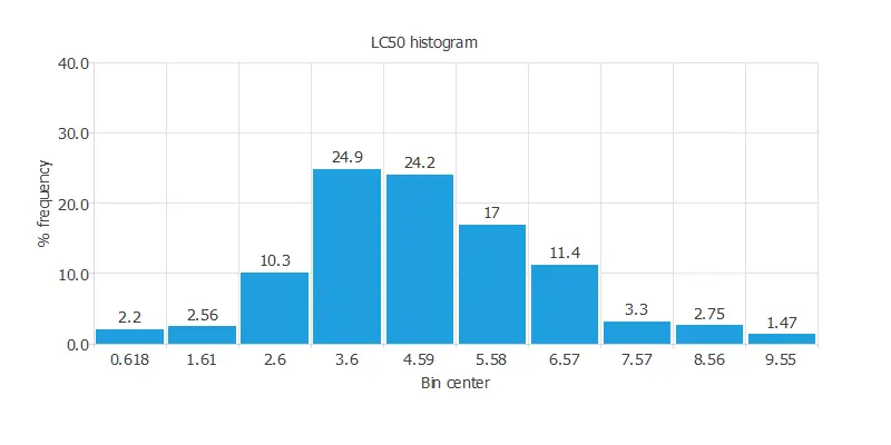
Variables distributions
Calculating the data distributions helps us check for the correctness of the available information and detect anomalies. The following chart shows the histogram for the power-generated variable:
Inputs-targets correlations
It is also interesting to look for dependencies between input and target variables. To do that, we can plot an inputs-targets correlations chart.
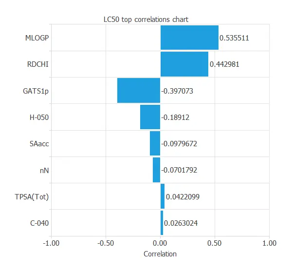
MLOGP and RDCHI are the most correlated variables because they measure lipophilicity, which is the driving force of narcosis.
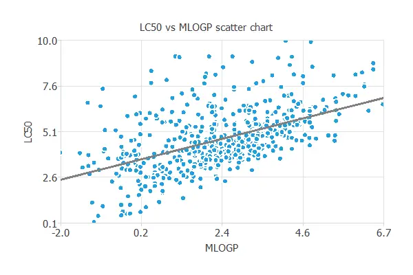
Scatter charts
In a scatter chart, we can visualize how this correlation works.
3. Neural network
The second step is building a neural network representing the approximation function. It is usually composed by:
- Scaling layer.
- Perceptron layers.
- Unscaling layer.
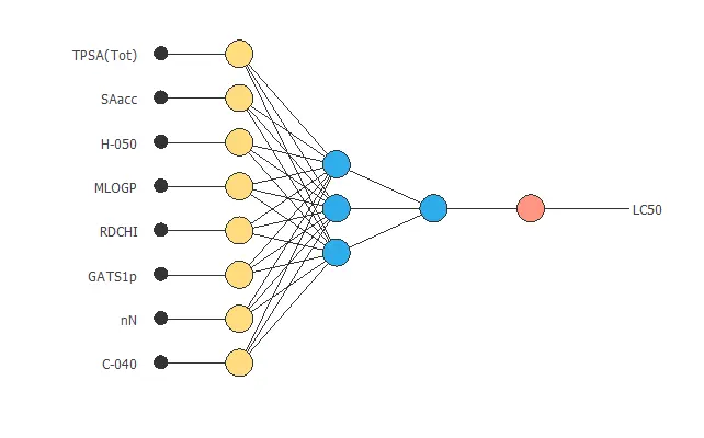
The neural network has 8 inputs (TPSA, SAacc, H-050, MLOGP, RDCHI, GATS1p, nN, C-040) and 1 output (LC50).
The scaling layer contains the statistics of the inputs. We use the automatic setting for this layer to accommodate the best scaling technique for our data.
We use 2 perceptron layers here:
- The first perceptron layer has 8 inputs, 3 neurons, and a hyperbolic tangent activation function.
- The second perceptron layer has 3 inputs, 1 neuron, and a linear activation function.
The unscaling layer contains the statistics of the outputs. We use the automatic method as before.
The following graph represents the neural network for this example.
4. Training strategy
The fourth step is to select an appropriate training strategy. It is composed of two parameters:
- Loss index.
- Optimization algorithm.
The loss index defines what the neural network will learn. It is composed of an error term and a regularization term.
The error term chosen is the normalized squared error. It divides the squared error between the neural network outputs and the data set’s targets by its normalization coefficient. If the normalized squared error has a value of 1, then the neural network predicts the data ‘in the mean,’ while a value of zero means a perfect data prediction. This error term does not have any parameters to set.
The regularization term is the L2 regularization. It is applied to control the neural network’s complexity by reducing the parameters’ value. We use a weak weight for this regularization term.
The optimization algorithm is in charge of searching for the neural network parameters that minimize the loss index.
Here, we chose the quasi-Newton method as an optimization algorithm.
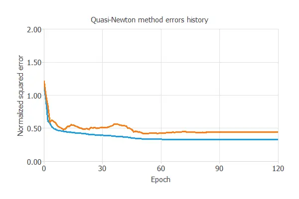
The following chart shows how the training (blue) and selection (orange) errors decrease with the epochs during the training process. The final values are training error = 0.331 NSE and selection error = 0.481 NSE, respectively.
Even though we are getting moderately good results, our model is far from perfect, mainly because of the small size of the Data Set we are working with. This might be one of the most significant issues of Machine Learning.
5. Model selection
In this case, Model selection algorithms aren’t beneficial to improve our model’s performance, as having a more complex architecture can also broaden the small Data Set problem.
6. Testing analysis
The purpose of the testing analysis is to validate the generalization capabilities of the neural network. We use the testing instances in the data set, which have never been used before.
A standard testing method in approximation applications is to perform a linear regression analysis between the predicted and the real pollutant level values.
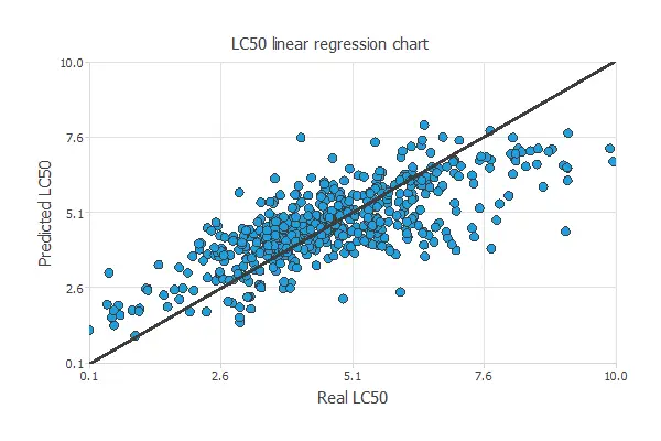
For a perfect fit, the correlation coefficient R2 would be 1. Considering our small Data Set issues, we have R2 = 0.744, so the neural network predicts the testing data quite well.
We have achieved a mean error of 8.64%.
7. Model deployment
In the model deployment phase, the neural network predicts outputs for inputs it has never seen.
We can calculate the neural network outputs for a given set of inputs:
- TPSA(Tot): 48.473.
- SAacc: 58.869.
- H-050: 0.938.
- MLOGP: 2.313.
- RDCHI: 2.492.
- GATS1p: 1.046.
- nN: 1.004.
- C-040: 0.3534.
- LC50: 4.92.
For that purpose, we can use Response Optimization. The objective of the response optimization algorithm is to exploit the mathematical model to look for optimal operating conditions. Indeed, the predictive model allows us to simulate different operating scenarios and adjust the control variables to improve efficiency.
An example is to minimize LC50 toxicity while maintaining the number of nitrogen atoms equal to the desired value.
The following table resumes the conditions for this problem.
| Variable name | Condition | |
|---|---|---|
| TPSA(Tot) | None | |
| SAacc | None | |
| H-050 | None | |
| MLOGP | None | |
| RDCHI | None | |
| GATS1p | None | |
| nN | Equal to | 2 |
| C-040 | None | |
| LC50 | Minimize |
The following list shows the optimum values for previous conditions.
- TPSA(Tot): 93.6666.
- SAacc: 345.496.
- H-050: 1.17883.
- MLOGP: -4.5905.
- RDCHI: 4.53847.
- GATS1p: 1.30937.
- nN: 2.
- C-040: 6.24457.
- LC50: 0.18981.
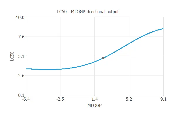
Directional outputs plot the neural network outputs through some reference points.
The following list shows the reference points for the plots.
- TPSA(Tot): 48.473.
- SAacc: 58.869.
- H-050: 0.938.
- MLOGP: 2.313.
- RDCHI: 2.492.
- GATS1p: 1.046.
- nN: 1.004.
- C-040: 0.3534.
We can see here how MLOGP affects LC50:
The mathematical expression represented by the predictive model is displayed next:
            scaled_TPSA(Tot) = TPSA(Tot)*(1+1)/(347.3200073-(0))-0*(1+1)/(347.3200073-0)-1;
scaled_SAacc = SAacc*(1+1)/(571.9520264-(0))-0*(1+1)/(571.9520264-0)-1;
scaled_H-050 = H-050*(1+1)/(18-(0))-0*(1+1)/(18-0)-1;
scaled_MLOGP = MLOGP*(1+1)/(9.147999763-(-6.446000099))+6.446000099*(1+1)/(9.147999763+6.446000099)-1;
scaled_RDCHI = RDCHI*(1+1)/(6.43900013-(1))-1*(1+1)/(6.43900013-1)-1;
scaled_GATS1p = GATS1p*(1+1)/(2.5-(0.2809999883))-0.2809999883*(1+1)/(2.5-0.2809999883)-1;
scaled_nN = nN*(1+1)/(11-(0))-0*(1+1)/(11-0)-1;
scaled_C-040 = C-040*(1+1)/(11-(0))-0*(1+1)/(11-0)-1;
perceptron_layer_output_0 = tanh[ 0.291703 + (scaled_TPSA(Tot)*-0.391549)+ (scaled_SAacc*0.251752)+ (scaled_H-050*0.085857)+ (scaled_MLOGP*-0.277858)+ (scaled_RDCHI*-1.14629)+ (scaled_GATS1p*0.803457)+ (scaled_nN*-0.240904)+ (scaled_C-040*-0.137404) ];
perceptron_layer_output_1 = tanh[ 0.240456 + (scaled_TPSA(Tot)*0.895344)+ (scaled_SAacc*-0.575449)+ (scaled_H-050*0.216825)+ (scaled_MLOGP*0.676507)+ (scaled_RDCHI*0.277635)+ (scaled_GATS1p*-0.115849)+ (scaled_nN*-0.0410888)+ (scaled_C-040*-0.239895) ];
perceptron_layer_output_2 = tanh[ 1.35559 + (scaled_TPSA(Tot)*0.868684)+ (scaled_SAacc*-0.00789895)+ (scaled_H-050*0.878771)+ (scaled_MLOGP*0.816033)+ (scaled_RDCHI*-2.5133)+ (scaled_GATS1p*2.02157)+ (scaled_nN*-0.148986)+ (scaled_C-040*-1.02231) ];perceptron_layer_output_0 = [ -0.309113 + (perceptron_layer_output_0*2.07224)+ (perceptron_layer_output_1*2.20069)+ (perceptron_layer_output_2*-1.55368) ];unscaling_layer_output_0 = perceptron_layer_output_0*(10.04699993-0.1220000014)/(1+1)+0.1220000014+1*(10.04699993-0.1220000014)/(1+1);
References
- M. Cassotti, D. Ballabio, V. Consonni, A. Mauri, I. V. Tetko, R. Todeschini (2014). Prediction of acute aquatic toxicity towards daphnia magna using GA-kNN method, Alternatives to Laboratory Animals (ATLA), 42,31:41.