Introduction
Machine learning can help physicians predict lung cancer recurrence, enabling earlier interventions and personalized treatment.
Recurrence after surgery is a major challenge, making accurate risk assessment essential for follow-up and therapy decisions.
We developed a neural network model using gene expression and clinical data to estimate 5-year relapse risk.
Using 335 patients (GEO dataset), the model achieved an AUC of 0.84 and 76.3% accuracy, demonstrating strong potential as a clinical decision-support tool.
Healthcare professionals can test this methodology by downloading Neural Designer.
Contents
The following index outlines the steps for performing the analysis.
1. Model type
- Problem type: Binary classification (lung relapse or no relapse)
- Goal: Model the probability of lung relapse based on gene expression and clinical data using AI and machine learning to support clinical decision-making.
2. Data set
Data source
The lung_cancer_relapse.csv file has the data for this example.
The target variable can only be binary in a classification model: 0 (false, no) or 1 (true, yes).
The number of rows (instances) in the data set is 18388, and the number of columns (variables) is 11747.
Variables
The following list summarizes the variables used in the lung cancer relapse model:
Clinical features
month (0–60) – Time from the patient’s surgical procedure until month 60 (5 years).
source_name – Hospital source of the sample.
sex – Male or female.
age_in_months – Age of the patient in months.
race – Patient race, categorized by shared physical traits.
clinical treatment adjuvant chemotherapy (0/1) – Whether or not the patient received chemotherapy.
clinical treatment adjuvant radiotherapy (0/1) – Whether or not the patient received radiotherapy.
pathological_nodes (0, 1, 2+) – Lymph node involvement relative to the TNM classification.
pathological_tumour (1–4) – Extent of the primary tumor relative to the TNM classification.
smoking_history (0/1) – Patient smoking history.
surgical_margins – Margin of non-tumorous tissue around the resected tumor.
histologic_grade (0–2) – Description of how abnormal the cancer cells/tissue look under a microscope.
Gene expression features
- RAD51, ADGRF5, COCH, SLC2A1, CLU, ZDHHC7, LRFN4, AP2A2 – Expression levels of selected genes significantly correlated with lung cancer relapse.
Target variable
relapse (yes or no) – 0 = no relapse, 1 = patient experienced lung cancer relapse within 5 years.
Instances
The dataset’s instances (one per patient, including input and target variables) are split into training (60%), validation (20%), and testing (20%) subsets by default, adjustable as needed.
Variables distributions
The distributions of all variables can be analyzed; the figure shows a pie chart of patients with and without relapse.
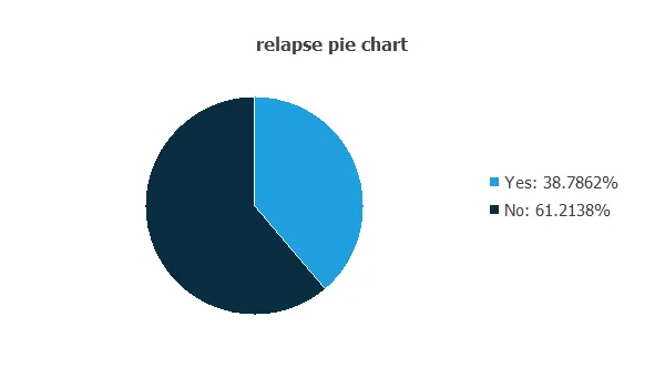
As depicted in the image, 38.79% of patients experienced a relapse, while 61.21% did not.
Input-target correlations
The input-target correlations indicate which clinical and pathological factors most influence whether a patient will experience a relapse, making them particularly relevant for our analysis.
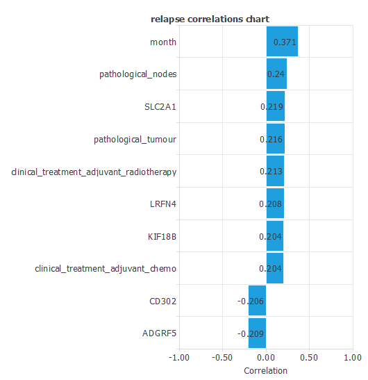
Here, the most correlated variables with relapse are month, pathological nodes, and SLC2A1.
3. Neural network
A neural network is an artificial intelligence model inspired by how the human brain processes information.
It is organized in layers: the input layer receives the variables, and the output layer provides the probability of belonging to a given class.
Trained with historical data, the network learns to recognize patterns and distinguish between categories, offering objective support for decision-making.
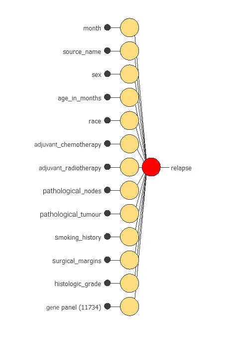
The network uses thirteen clinical and pathological variables to predict the probability of cancer relapse, with connections showing each variable’s contribution.
4. Training strategy
Training a neural network uses a loss function to measure errors and an optimization algorithm to adjust the model, ensuring it learns from data while avoiding overfitting for good performance on new cases.
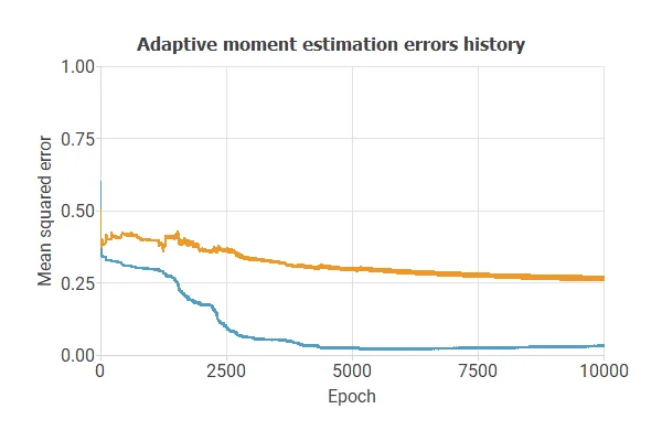
The model was trained for accuracy and stability on new data, with training and selection errors decreasing steadily (0.03 and 0.27 MSE), indicating effective learning and generalization.
5. Model selection
The objective of model selection is to find the network architecture that minimizes the error, that is, with the best generalization properties for the selected instances of the data set.
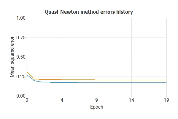
After multiple simulations, the optimal model achieved a training error of 0.17 NSE and a selection error of 0.20 NSE, showing improved performance on unseen samples.
Also, we have reduced the number of inputs to only 11 features. Our network is now like this:
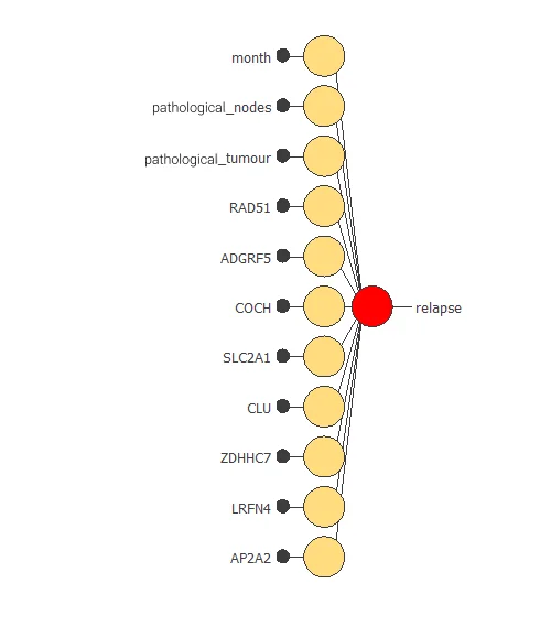
Our final network has 11 inputs corresponding to month, pathological_nodes, pathological_tumour, RAD51, ADGRF5, COCH, SLC2A1, CLU, ZDHHC7, LRFN4, and AP2A2.
6. Testing analysis
The testing analysis aims to validate the performance of the generalization properties of the trained neural network.
ROC curve
The ROC curve is a standard tool to evaluate a classification model, showing how well it distinguishes between two classes by comparing predicted results with actual outcomes, such as relapse or no relapse in lung cancer patients.
A random classifier scores 0.5, while a perfect classifier scores 1.
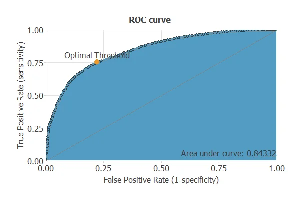
The model achieves an AUC of 0.843, demonstrating excellent performance in distinguishing patients who will experience a relapse from those who will not.
Confusion matrix
The confusion matrix shows the model’s performance by comparing predicted and actual relapse outcomes. It includes:
True positives – patients correctly predicted to experience a relapse
False positives – patients incorrectly predicted to experience a relapse
False negatives – patients incorrectly predicted not to experience a relapse
True negatives – patients correctly predicted not to experience a relapse
For a decision threshold of 0.5, the confusion matrix was:
| Predicted positive | Predicted negative | |
|---|---|---|
| Real positive | 18 | 8 |
| Real negative | 8 | 33 |
In this case, 76% cases were correctly classified and 24% were misclassified.
Binary classification
The performance of this binary classification model is summarized with standard measures.
Accuracy: 76.31% of patients were correctly classified regarding relapse.
Error rate: 23.68% of cases were misclassified.
Sensitivity: 75.21% of patients who relapsed were correctly identified.
Specificity: 77.78% of patients who did not relapse were correctly identified.
These measures indicate that the model is highly effective at predicting lung cancer relapse.
7. Model deployment
After confirming the neural network’s ability to generalize, the model can be saved for future use in deployment mode.
This allows the trained network to be applied to new patients, using their clinical variables to calculate the probability of lung cancer relapse.
In deployment mode, healthcare professionals can use the model as a reliable diagnostic support tool for classifying new patients.
The Neural Designer software exports the trained model automatically, making it easy to integrate into clinical practice.
Conclusions
The lung cancer recurrence prediction model (GEO data) achieved AUC = 0.84, accuracy = 76.3% for 5-year relapse prediction.
Top predictors—pathological nodes, tumor stage, and gene markers (SLC2A1, RAD51)—match established clinical and molecular factors.
The model can support risk stratification, follow-up, and treatment planning in clinical practice.