Introduction
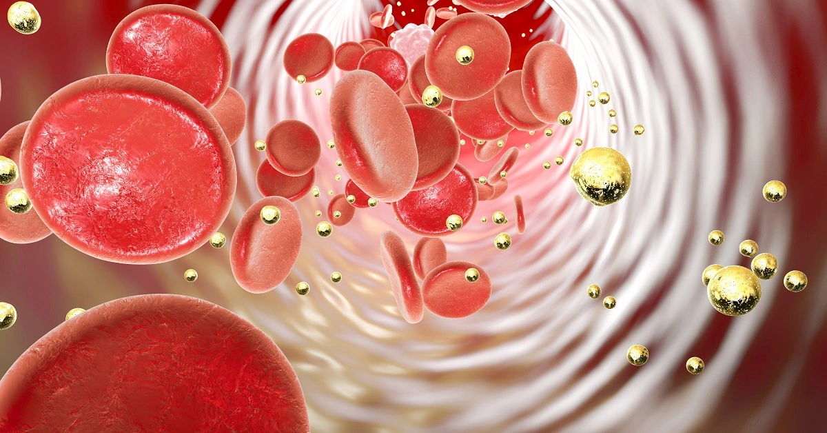
Nanoparticle-based machine learning can predict their vascular behavior, particularly adhesion to vessel walls, which is crucial for diagnosis, treatment, and medical imaging.
Predicting nanoparticle adhesion under varying blood flow is experimentally challenging.
This study used a neural network with particle diameter and shear rate, achieving high correlation (0.946) and low error (0.098), showing strong potential for vascular applications.
This approach can be explored using Neural Designer
Contents
The following index outlines the steps for performing the analysis.
1. Model type
- Problem type: Regression (continuous adhesive strength)
- Goal: Model the adhesive strength as a function of shear rate and particle diameter to support vascular nanoparticle design using artificial intelligence and machine learning.
2. Data set
Data source
The dataset (58 instances, 3 variables): two inputs (shear_rate, particle_diameter) and one target (particles_adhering).
Variables
The following list summarizes the variables’ information:
Experimental conditions
- shear_rate (1/s) – Wall shear rate applied to the nanoparticle; higher values represent stronger flow conditions in the vascular system.
Particle properties
- particle_diameter (µm) – Diameter of each nanoparticle; larger particles tend to exhibit stronger adhesive behavior.
Target variable
particles_adhering (count/area) – Number of particles adhering per unit area to the collagen substrate, representing adhesive strength.
Instances
The dataset’s instances are split into training (60%), validation (20%), and testing (20%) subsets by default.
You can adjust them as needed.
Variables distributions
Also, we can examine the distributions for all variables. The figure shows adhesive strength and its correlations with the input variables.
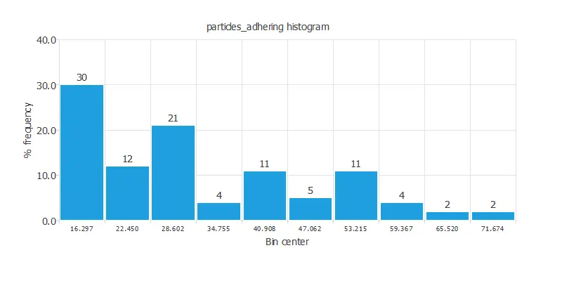
As we can see, the correlations are positive with particle diameter and negative with shear rate.
Input-target correlations
The input-target correlations indicate which factors most influence adhesive strength and, therefore, are more relevant to our analysis.
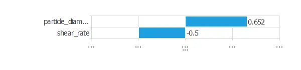
Here, the variables most correlated with adhesive strength are particle diameter and shear rate.
3. Neural network
A neural network is an artificial intelligence model inspired by how the human brain processes information.
It is organized in layers: the input layer receives the variables, the hidden layers combine them to detect relevant patterns, and the output layer provides the probability of belonging to a given class.
Trained with historical data, the network learns to recognize patterns and distinguish between categories, offering objective support for decision-making.
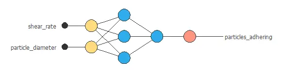
The network combines two nanoparticle-related variables through two hidden layers to predict adhesive strength, with connections showing each variable’s contribution.
4. Training strategy
Training a neural network involves defining a loss function and optimization algorithm to learn from data while avoiding overfitting, ensuring good performance on both training and new cases.
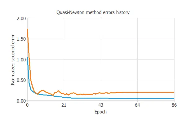
The model was trained to ensure accuracy and stability on new data, with training and validation errors decreasing (0.062 NSE and 0.098 NSE), showing effective learning and generalization to new nanoparticle cases.
5. Testing analysis
After training, the model’s predictive capacity is tested by comparing its outputs to target values on unseen data, determining if it is ready for production.
Linear regression
The next chart illustrates the linear regression analysis for the variable particles_adhering.
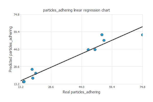
For a perfect fit, intercept, slope, and correlation should be 0, 1, and 1. Here, with intercept = -2.57, slope = 1.11, and correlation = 0.946, the model performs well, close to ideal values.
6. Model deployment
Once the neural network’s generalization is confirmed, it can be saved and deployed to predict adhesive strength from shear rate and particle diameter.
In deployment mode, researchers can use it to simulate and optimize nanoparticle design, with Neural Designer exporting the model for easy integration into lab or clinical workflows.
Conclusions
The machine learning model accurately predicted nanoparticle adhesive strength (correlation = 0.946, error = 0.098) using particle diameter and shear rate.
Larger particles adhered more strongly, while higher shear reduced adhesion, consistent with vascular physiology.
This approach provides a reliable tool for optimizing nanoparticle design in drug delivery, imaging, and diagnostics, reducing experimental testing and accelerating development.
References
- “Optimizing particle size for targeting diseased microvasculature: from experiments to artificial neural networks“, Daniela P Boso, Sei-Young Lee, Mauro Ferrari, Bernhard A Schrefler, Paolo Decuzzi. International Journal of Nanomedicine, 2011.