This example uses machine learning to build a digital twin of an electric motor.

The advance of new technology and electric cars has been taking place recently. As a result, many companies want to ensure their electric engines are the best in the market regarding reliability, autonomy for the client, and durability. Therefore, these companies perform tests digitally to prevent any damage to the actual product and find the best temperature interval in which the engines work the best.

Performance optimization can be applied to understand the behavior of the electric motors. We have gathered an extensive data set of several sensor data collected from a permanent magnet synchronous motor deployed on a test bench for this study. Robust rotor and stator temperature estimators help the automotive industry improve their motors, reducing power losses and, eventually, heat build-up.

1. Application type

This is an approximation project since the variable to be predicted is continuous (engine temperature).

The fundamental goal is understanding how voltage and current affect numerous car features and the temperature of different parts of an electric motor.

2. Data set

The first step is to prepare the data set, which is the source of information for the approximation problem. It is composed of:

• Data source.
• Variables.
• Instances.

Data source

The file permanent_magnet_synchronous_motor.csv contains the data for this example. Here, the number of variables (columns) is 14, and the number of instances (rows) is 107.

Variables

In that way, this problem has the following variables:

• temperature_ambient, ambient temperature measured by a thermal sensor located close to the stator.
• temperature_coolant, coolant temperature. The motor is water-cooled. Measurement is taken at the outflow.
• voltage_direct, voltage d-component.
• voltage_quadrature, voltage q-component.
• current_direct, current d-component
• current_quadrature, current q-component.
• voltage_module, vector module from the d-q voltage components.
• current_module, vector module from the d-q current components.
• speed_motor, vehicle motor speed.
• torque, torque induced by current.
• temperature_stator_yoke, stator yoke temperature measured with a thermal sensor.
• temperature_stator_tooth, stator tooth temperature measured with a thermal sensor.
• temperature_stator_winding, stator winding temperature measured with a thermal sensor.

We have different variables in the study: ‘temperature_ambient’, ‘temperature_coolant’, ‘voltage_direct’, ‘voltage_quadrature’, ‘current_direct’, ‘current_quadrature’, ‘u_module’, and ‘i_module’ are inputs. On the contrary, ‘motor_speed’, ‘torque’, ‘stator_yoke’, stator_tooth’, and ‘stator_winding’ are the targets of this study. Indeed, our main goal is to describe the behavior of the electric motor to prevent overheating. That is why these output variables show the temperature of the engine’s internal parts.

Instances

They are divided randomly into training, selection, and testing subsets, containing 60%, 20%, and 20% of the instances, respectively. More specifically, 65 samples are used here for training, 21 for validation, and 21 for testing.

Variables distribution

Once we establish the data set information, we perform analytics to check the data quality.

For instance, we can calculate the data distribution. The next figure depicts the histogram for one of the target variables.

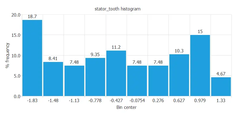
In this diagram, we can see a normal distribution of the stator tooth temperature representing one of the parts of the stator temperature. We could affirm it is normal because this output simultaneously depends on many input variables. During this experiment, the inputs constantly varied, causing the targets to have this type of distribution.

Inputs-targets correlations

The next figure depicts inputs-targets correlations. This might help us see the different inputs’ influence on the motor temperature.

As this machine learning study has various target variables, we show the correlations diagram of one.

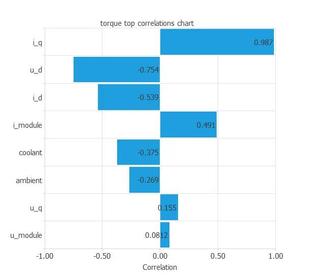
The above chart shows that a few instances have a critical dependency on the variable ‘torque’. As we can see, an instance is highly correlated to this target, which is the case of the input ‘current_quadrature’.

At first sight, we could have predicted this behavior simply by looking at the data set and realizing the torque is induced by the current, in this case, by the quadrature coordinate of the current.

Scatter charts

We can also plot a scatter chart with the stator winding temperature versus the ambient temperature.

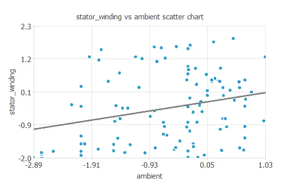
Logically, the more the ambient temperature, the more stator winding temperature.

3. Neural network

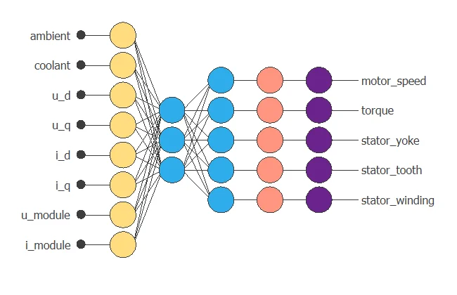
The neural network outputs the different motor temperatures as a function of the current, voltage, coolant, and ambient temperature.

Approximation models usually contain the following layers:

• Scaling layer.
• Perceptron layers.
• Unscaling layer.

The scaling layer transforms the original inputs to normalized values. Here, we set the mean and standard deviation scaling method so that the input values have a mean of 0 and a standard deviation of 1.

Here, two perceptron layers are added to the neural network. This number of layers is enough for most applications. The first layer has eight inputs and three neurons. The second layer has three inputs and five neurons.

The unscaling layer transforms the normalized values from the neural network into the original outputs. Here, we also use the mean and standard deviation unscaling method.

The next figure shows the resulting network architecture.

4. Training strategy

The next step is selecting an appropriate training strategy to define what the neural network will learn. A general training strategy is composed of two concepts:

• A loss index.
• An optimization algorithm.

The loss index chosen is the normalized squared error with L2 regularization. This loss index is the default in approximation applications.

The optimization algorithm chosen is the quasi-Newton method. This optimization algorithm is the default for medium-sized applications like this one.

Once the strategy has been set, we can train the neural network. The following chart shows how the training (blue) and selection (orange) errors decrease with the training epoch during the training process.

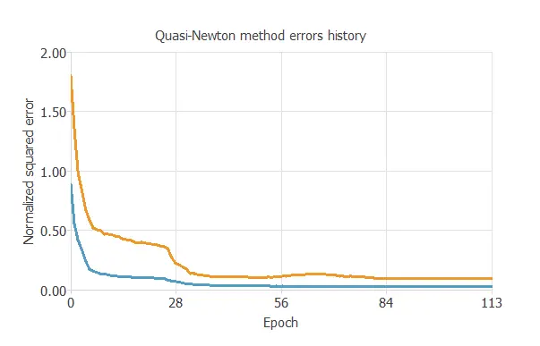
The most critical training result is the final selection error. Indeed, this is a measure of the generalization capabilities of the neural network. Here, the final selection error is selection error = 0.083 NSE.

5. Model selection

The objective of model selection is to find the network architecture with the best generalization properties. We want to improve the final selection error obtained before (0.083 NSE).

The best selection error is achieved using a model whose complexity is the most appropriate to produce a good data fit. Order selection algorithms are responsible for finding the optimal number of perceptrons in the neural network.

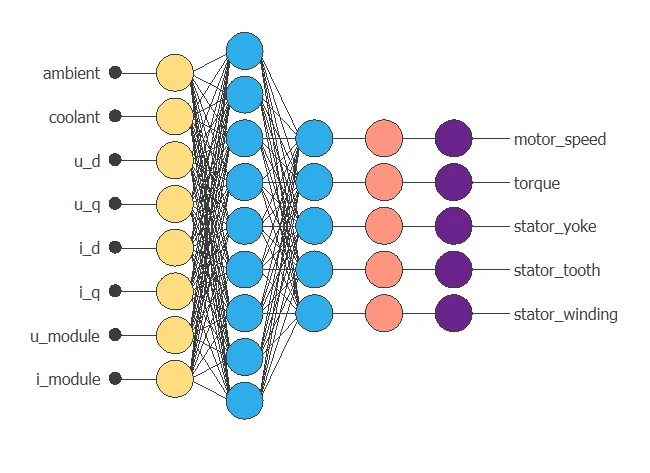
The final training error continuously decreases with the number of neurons. However, the final selection error takes a minimum value at some point. Here, the optimal number of neurons is 9, corresponding to a selection error of 0.0432.

The following figure shows the optimal network architecture for this application.

6. Testing analysis

The objective of the testing analysis is to validate the generalization performance of the trained neural network. The testing compares the values provided by this technique to the observed values.

A standard testing technique in approximation problems is to perform a linear regression analysis between the predicted and the real values using an independent testing set. The following figure illustrates a graphical output provided by this testing analysis.

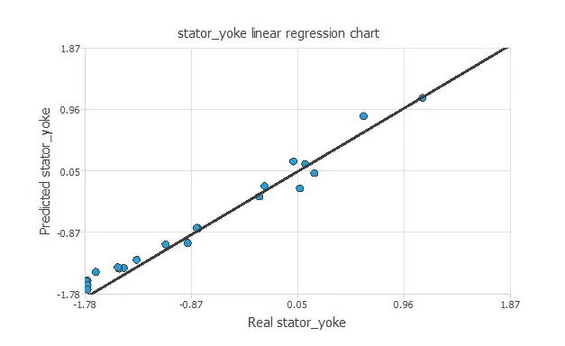
The above chart shows that the neural network is predicting the entire range of temperature data well. The correlation value is    R2 = 0.990, indicating the model has a reliable prediction capability.

7. Model deployment

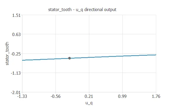
We can plot a directional output of the neural network to see how the targets vary with a given input for all other fixed inputs.
The next plot shows the stator tooth temperature as a function of the quadrature coordinate of the voltage through the following point:

• temperature_ambient: -0.603. (scaled: Mean=0, Deviation=1)
• temperature_coolant: -0.393. (scaled: Mean=0, Deviation=1)
• voltage_direct: -0.359. (scaled: Mean=0, Deviation=1)
• voltage_quadrature: -0.235. (scaled: Mean=0, Deviation=1)
• current_direct: 0.0834. (scaled: Mean=0, Deviation=1)
• current_quadrature: 0.231. (scaled: Mean=0, Deviation=1)
• voltage_module: 1.26. (scaled: Mean=0, Deviation=1)
• current_module: 1.19. (scaled: Mean=0, Deviation=1)

The electric_motor.py contains the Python code for the electric motor temperature Neural Network.

References

• Kaggle Machine Learning Repository. Electric Motor Temperature Data Set.

Related posts