A combined-cycle power plant comprises gas turbines, steam turbines, and heat recovery steam generators.
In this type of plant, electricity is generated by combining gas and steam turbines in a single cycle.
Then, it is transferred from one turbine to another.
This process involves the emission of certain gas pollutants, such as NOx (nitrogen oxides), which are harmful to human health.
Predicting peaks in such emissions might give us a chance to implement preventive measures.
This example models NOx levels to provide essential information about the power plant’s emissions and to help reduce them.
Contents
- Application type.
- Data set.
- Neural network.
- Training strategy.
- Model selection.
- Testing analysis.
- Model deployment.
This example is solved with Neural Designer. You can use the free trial to understand how the solution is achieved step by step.
1. Application type
This is an approximation project since the variable to be predicted is continuous (NOx emission levels).
The primary objective is to model pollutant emissions as a function of environmental and control variables.
2. Data set
The data set contains three concepts:
- Data source.
- Variables.
- Instances.
Data source
The data file power_plant_gas_emissions.csv contains 36,733 samples with 11 variables, aggregated over one hour, from a gas turbine located in Turkey’s northwestern region between 2011 and 2015.
Variables
Ambient conditions
- ambient_temperature – Ambient temperature (°C).
- ambient_pressure – Ambient pressure (mbar).
- ambient_humidity – Ambient humidity (%).
Air intake & compression
- air_filter_difference_pressure – Pressure difference across the air filter (mbar).
- compressor_discharge_pressure – Pressure of gases expelled by the compressor (mbar).
Combustion & turbine process
- gas_turbine_exhaust_pressure – Pressure of exhaust gases from the combustion chamber (mbar).
- turbine_inlet_temperature – Exhaust gas temperature entering the turbine (°C).
- turbine_after_temperature – Exhaust gas temperature exiting the turbine (°C).
Targets
- turbine_energy_yield – Hourly energy yield of the turbine (MWh).
- NOx – Nitrogen oxides concentration in exhaust gases (mg/m³).
Instances
Variable distributions
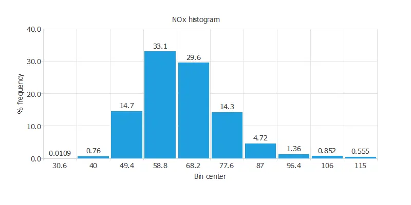
Calculating the data distributions helps us verify the accuracy of the available information and detect anomalies.
The following chart shows the histogram for the NOx variable.
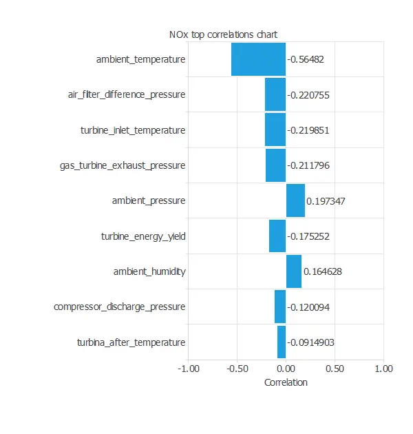
Input-target correlations
It is also interesting to look for dependencies between a single input and a single target variable.
To do that, we can plot an input-targets correlation chart.
For the NOx, we have:
Scatter charts
Next, we plot a scatter chart for the most significant correlations for our target variable.
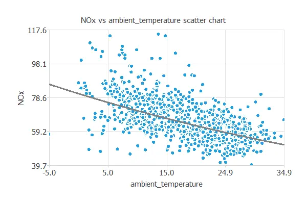
As we saw earlier, the higher the ambient temperature, the less gas is emitted by the power plant.
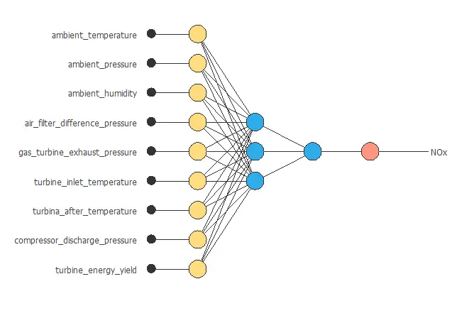
3. Neural network
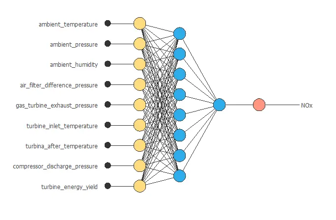
The second step is to build a neural network that represents the approximation function.
The neural network has nine inputs (ambient temperature, ambient pressure, ambient humidity, air filter difference pressure, gas turbine exhaust pressure, turbine inlet temperature, turbine after temperature, compressor discharge pressure) and two outputs (turbine energy yield and NOx).
Approximation models are usually composed of:
- Scaling layer.
- Perceptron layers.
- Unscaling layer.
Scaling layer
The scaling layer contains the statistics of the inputs. We use the automatic setting for this layer to accommodate the best scaling technique for our data.
Dense layers
We use two perceptron layers here:
- The first perceptron layer has 9 inputs, 3 neurons, and a hyperbolic tangent activation function.
- The second perceptron layer has 3 inputs, 2 neurons, and a linear activation function.
Unscaling layer
The unscaling layer contains the statistics of the outputs. We use the automatic method as before.
The next graph represents the neural network for this example.
4. Training strategy
The fourth step is to select an appropriate training strategy. It is composed of two parameters:
- Loss index.
- Optimization algorithm.
Loss index
The loss index defines what the neural network will learn. It is composed of an error term and a regularization term.
The error term chosen is the normalized squared error. It divides the squared error between the neural network’s outputs and the targets in the data set by its normalization coefficient.
If the normalized squared error has a value of 1, then the neural network is predicting the data ‘in the mean’, while a value of zero means a perfect prediction of the data. This error term has no parameters to set.
The regularization term is the L2 regularization. It is applied to control the complexity of the neural network by reducing the value of the parameters. We use a weak weight for this regularization term.
Optimization algorithm
The optimization algorithm searches for the neural network parameters that minimize the loss index. Here, we chose the quasi-Newton method as the optimization algorithm.
The chart below shows how training error (blue) and selection error (orange) decrease as the number of epochs increases.
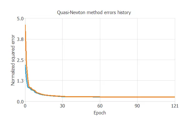
The final values are training error = 0.260 NSE and selection error = 0.263 NSE, respectively.
5. Model selection
The objective of model selection is to find the network architecture with the best generalization properties.
We aim to reduce the final selection error obtained previously (0.263 NSE).
The best selection error is achieved using a model with the most appropriate complexity to produce a good data fit.
Order selection algorithms are responsible for finding the optimal number of perceptrons in the neural network.
The following chart shows the results of the incremental order algorithm.
The blue line shows training error and the orange line shows selection error, both as functions of the number of neurons.
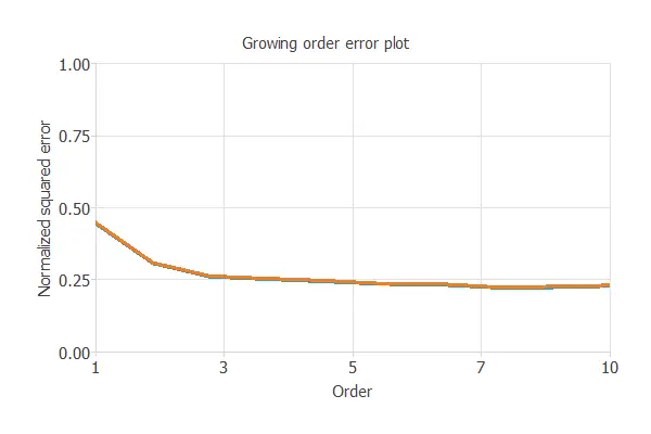
As we can see, the final training error continuously decreases with the number of neurons. However, the final selection error takes a minimum value at some point. Here, the optimal number of neurons is 8, corresponding to a selection error of 0.224 NSE.
The following figure shows the optimal network architecture for this application.
6. Testing analysis
The purpose of the testing analysis is to validate the generalization capabilities of the neural network.
We use the testing instances in the data set, which have never been used before.
Goodness-of-fit
A standard testing method in approximation applications is to perform a linear regression analysis between the predicted and the real pollutant level values.
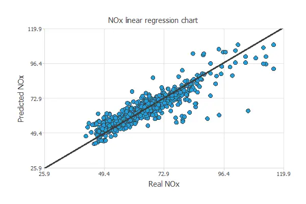
For a perfect fit, the correlation coefficient R2 would be 1. With R2 = 0.889, the neural network accurately predicts the testing data.
7. Model deployment
In the model deployment phase, the neural network is used to predict outputs for inputs that it has not seen before.
Outputs
We can calculate the neural network outputs for a given set of inputs:
- ambient_temperature: 17.713 degrees Celsius.
- ambient_pressure: 1013.07 millibars.
- ambient_humidity: 77.867 %.
- air_filter_difference_pressure: 3.926 millibars.
- gas_turbine_exhaust_pressure: 25.56 millibars.
- turbine_inlet_temperature: 1081.44 degrees Celsius.
- turbine_after_temperature: 546.161 degrees Celsius.
- compressor_discharge_pressure: 133.506 millibars.
- turbine_energy_yield: 12.061 Megawatts per hour.
- NOx: 67.518 milligrams per cubic meter.
Response optimization
You can also use Response Optimization, which applies the predictive model to find the best operating conditions by simulating scenarios and adjusting control variables to improve efficiency.
An example is to minimize gas turbine exhaust pressure while maintaining the NOx level below the desired value.
The following table summarizes the conditions for this problem.
| Variable name | Condition | |
|---|---|---|
| Ambient temperature | None | |
| Ambient pressure | None | |
| Ambient humidity | None | |
| Air filter difference pressure | None | |
| Gas turbine exhaust pressure | Minimize | |
| Turbine inlet temperature | None | |
| Turbine after temperature | None | |
| Compressor discharge pressure | None | |
| Turbine energy yield | None | |
| NOx | Less than or equal to | 80 |
The next list shows the optimum values for the previous conditions.
- ambient_temperature: 21.2745 degrees Celsius.
- ambient_pressure: 1033.75 millibars.
- ambient_humidity: 53.3598 %.
- air_filter_difference_pressure: 6.02753 millibars.
- gas_turbine_exhaust_pressure: 17.8926 millibars.
- turbine_inlet_temperature: 1008.55 degrees Celsius.
- turbine_after_temperature: 515.503 degrees Celsius.
- compressor_discharge_pressure: 136.975 millibars.
- turbine_energy_yield: 15.0443 Megawatts per hour.
- NOx: 40.7311 milligrams per cubic meter.
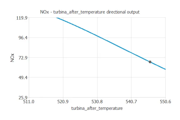
Directional outputs
Directional outputs plot the neural network outputs through some reference points.
The next list shows the reference points for the plots.
- ambient_temperature: 17.713 degrees Celsius.
- ambient_pressure: 1013.07 millibars.
- ambient_humidity: 77.867 %.
- air_filter_difference_pressure: 3.926 millibars.
- gas_turbine_exhaust_pressure: 25.56 millibars.
- turbine_inlet_temperature: 1081.44 degrees Celsius.
- turbine_after_temperature: 546.161 degrees Celsius.
- compressor_discharge_pressure: 133.506 millibars.
- turbine_energy_yield: 12.061 Megawatts per hour.
We can see here how the turbine inlet temperature affects NOx emissions:
Decreasing the turbine inlet temperature decreases NOx emissions.
This insight into our model can help us take preventive action against pollutant emissions.
For example, lowering the turbine inlet temperature by 10 °C cuts NOx emissions by about 16%, from 65 to 54 mg/m³.
We are using the turbine inlet temperature to reduce NOx levels because it is relatively easy to adjust its value.
However, by utilizing directional outputs, we can analyze any of our variables for this purpose.
References
- Heysem Kaya, Pinar Tufekci and Erdinç Uzun. ‘Predicting CO and NOx emissions from gas turbines: novel data and a benchmark PEMS’, Turkish Journal of Electrical Engineering & Computer Sciences, vol. 27, 2019, pp. 4783-4796