Introduction
Colon cancer is a leading cause of cancer-related deaths, and treatment outcomes depend on clinical and demographic factors. Selecting the right therapy after surgery is crucial to improving survival.
Using data from a randomized controlled trial of 607 patients treated with Levamisole plus Fluorouracil or chemotherapy, we implemented a neural network model to predict whether a patient survives at least five years after treatment.
This methodology highlights the potential of machine learning to support clinicians in tailoring treatments and improving patient outcomes.
Healthcare professionals can test it with Neural Designer’s trial version.
Contents
The following index outlines the steps for performing the analysis.
1. Model type
- Problem type: Binary classification (survived or deceased at five years)
- Goal: Model the probability of a patient surviving at least five years after treatment to support clinical decision-making.
2. Data set
Data source
The dataset coloncancer.csv includes 607 instances (rows) and 11 variables (columns), including an ID column.
Variables
The following list summarizes the variables’ information:
Demographic
sex (binary) – Male or female.
age (numeric) – Patient’s age at the beginning of the study.
Clinical features
obstruction (binary) – Obstruction of the colon by the tumor.
perforation (binary) – Perforation of the colon.
adherence (binary) – Tumor adheres to nearby organs.
nodes (numeric) – Number of affected lymph nodes.
more_than_4_nodes (binary) – Whether more than 4 lymph nodes are positive.
Treatment
- treatment (binary) – Treatment type: levamisole with fluorouracil or chemotherapy.
Tumor characteristics
differ_level (binary fields) – Differentiation level of the tumor:
Level 2: intermediate forms with both good and bad prognosis.
Level 3: tumors spread more easily, and the prognosis is worse.
extent_level (binary fields) – Extent of local spread:
Level 2: cancer has grown into the outer layers but not through them; no lymph node involvement; no distant spread.
Level 3: cancer has invaded the submucosa; spread to 4–6 nearby lymph nodes; no distant spread.
Level 4: cancer may have grown through the wall; may involve nearby nodes; has spread to one distant organ (e.g., liver or lung).
Target variable
survival (yes or no) – Patient survival within 5 years after treatment.
Instances
The dataset’s instances are split into training (60%), validation (20%), and testing (20%) subsets by default.
You can adjust them as needed.
Variables distributions
We can calculate variable distributions; the chart shows the number of survival and death cases in the dataset.
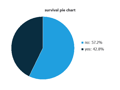
As depicted in the image, patients who survived represent 57.2% of the samples, while patients who did not survive account for approximately 42.8%.
We can also represent the distribution of the treatment variable:
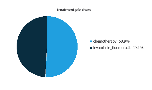
As depicted in the image, 50.9% of patients received chemotherapy, while 49.1% received levamisole combined with fluorouracil.
Input-target correlations
The input-target correlations indicate which clinical, demographic, or treatment factors most influence patient survival, and therefore are more relevant to our analysis.
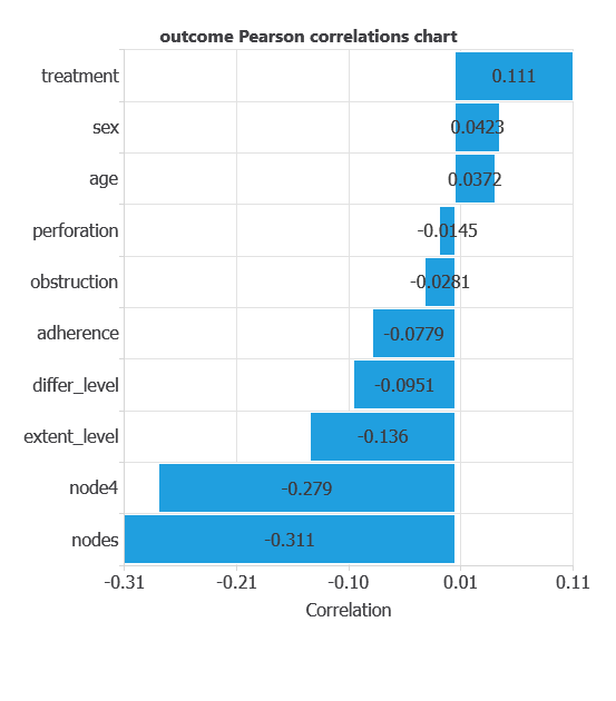
Here, the most correlated variables with with five-year survival outcome are nodes, node4, and treatment.
3. Neural network
A neural network is an artificial intelligence model inspired by how the human brain processes information.
It is organized in layers: the input layer receives the variables, and the output layer provides the probability of belonging to a given class.
Trained with historical data, the network learns to recognize patterns and distinguish between categories, offering objective support for decision-making.
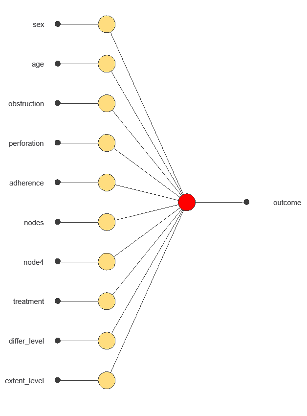
The network uses ten diagnostic variables to predict the probability of survival, with connections showing each variable’s contribution.
4. Training strategy
Training a neural network involves using a loss function to measure errors and an optimization algorithm to adjust the model, ensuring it learns from data while avoiding overfitting for good performance on new cases.
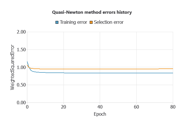
The model was trained for accuracy and stability, with training and selection errors decreasing steadily (0.836 and 0.954 WSE), indicating effective learning and generalization to new patients.
5. Testing analysis
We perform an exhaustive testing analysis to validate the generalization performance.
ROC curve
The ROC curve is a standard tool to evaluate a classification model, showing how well it distinguishes between two classes by comparing predicted results with actual outcomes, such as five-year survival (survived or deceased).
A random classifier scores 0.5, while a perfect classifier scores 1.
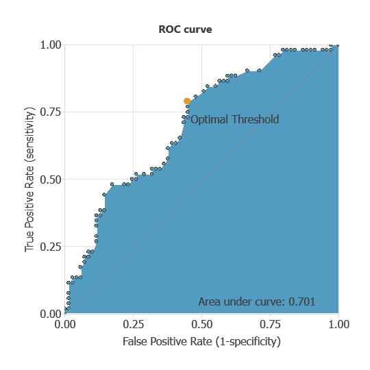
The model achieves an AUC of 0.701, demonstrating strong performance in distinguishing patients who survived from those who did not.
Confusion matrix
The confusion matrix shows the model’s performance by comparing predicted and actual outcomes. It includes:
True positives: patients correctly predicted to survive
False positives: patients incorrectly predicted to survive
False negatives: patients incorrectly predicted not to survive
True negatives: patients correctly predicted not to survive
For a decision threshold of 0.5, the confusion matrix was:
| Predicted positive | Predicted negative | |
|---|---|---|
| Real positive | 49 | 20 |
| Real negative | 25 | 27 |
In this case, 62.81% of cases were correctly classified and 37.19% were misclassified.
Binary classification
The performance of this binary classification tests model is summarized with standard measures.
Accuracy: 61.81% of patients were correctly classified.
Error rate: 37.2% of cases were misclassified.
Sensitivity: 71% of patients who survived were correctly identified.
Specificity: 51.19% of patients who did not survive were correctly identified.
These measures indicate that the model is highly effective at predicting five-year survival.
Directional outputs
Directional outputs were analyzed to assess five-year survival (alive vs. deceased) as a function of individual variables.
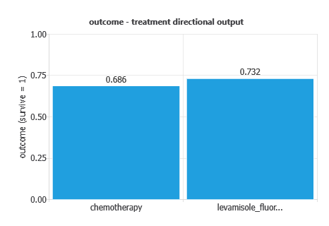
The graph shows survival probability by treatment: overall survival was 56.5%, 73.2% with Levamisole–Fluorouracil, and 68.6% with chemotherapy, indicating slightly better outcomes with the combination therapy.
6. Model deployment
After confirming the neural network’s ability to generalize, the model can be saved for future use in deployment mode.
This allows the trained network to be applied to new patients, using their clinical variables to calculate the probability of colon cancer.
In deployment mode, healthcare professionals can use the model as a reliable diagnostic support tool for classifying new patients.
The Neural Designer software exports the trained model automatically, making it easy to integrate into clinical practice.
Conclusions
- The colon cancer survival prediction model, trained on 607 patients, showed moderate but clinically meaningful performance (AUC = 0.701) in predicting five-year survival.
- Key factors—number of affected lymph nodes, >4 positive nodes, and treatment type—align with established oncology knowledge, supporting the model’s reliability.
- This study demonstrates how machine learning can complement traditional methods, helping oncologists with treatment decisions and survival assessment.
References
- We have obtained the data for this problem from Coursera.