In this example, we build a machine learning model to prognose diabetic retinopathy.
Diabetic retinopathy, also known as diabetic eye disease, is a medical condition that damages the retina due to diabetes.
Contents
- Application type.
- Data set.
- Neural network.
- Training strategy.
- Model selection.
- Testing analysis.
- Model deployment.
- Tutorial video.
This example is solved with Neural Designer. To follow it step by step, you can use the free trial.
1. Application type
The variable to be predicted can have two values (positive or negative on diabetic retinopathy). Thus, this is a binary classification project.
The goal here is to predict whether a patient will suffer from diabetic retinopathy conditioned on blood test features.
2. Data set
Data source
The diabetic_retinopathy.csv file contains the data for this application. Target variables can only have two values in a classification project type: 0 (false) or 1 (true). The number of instances (rows) in the data set is 6000, and the number of variables (columns) is 6.
Variables
The number of input variables, or attributes for each sample, is 3. All input variables are numerical values and represent the results of each test. The number of target variables is 1 and represents the presence or absence of retinopathy in each individual. The following list summarizes the information on the variables:
- age: (numeric).
- systolic_bp: (normal range: below 120mmHg). When the heart beats, it squeezes and pushes blood through the arteries to the rest of the body. This force creates pressure on the blood vessels, the systolic blood pressure.
- diastolic_bp: (normal range: lower than 80mmHg). It is the pressure in the arteries when the heart rests between beats. This is the time when the heart fills with blood and gets oxygen.
- cholesterol: (normal range: between 125 and 200 mg/dl). It is a waxy, fat-like substance found in every cell in the body.
- prognosis: (0 or 1). It is 1 if the patient has retinopathy and 0 if he doesn’t.
Instances
Finally, the use of all instances is set. Note that each instance contains a different patient’s input and target variables.
The data set is divided into training, validation, and testing subsets. 60% of the instances will be assigned for training, 20% for generalization, and 20% for testing. Specifically, 3600 are training samples, and 1200 are selection and testing examples.
Variables statistics
We can perform a few related analytics once the data set has been set. Subsequently, we check the provided information with these and ensure quality data.
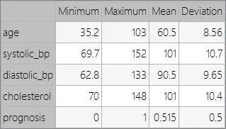
Furthermore, we can calculate the data statistics and draw a table with the minimums, maximums, means, and standard deviations of all attributes in the data set. The next table depicts these values.
Variables distributions
We can also calculate the distributions for all the variables. The following pie chart shows the number of patients with diabetic retinopathy and without it in the data set.
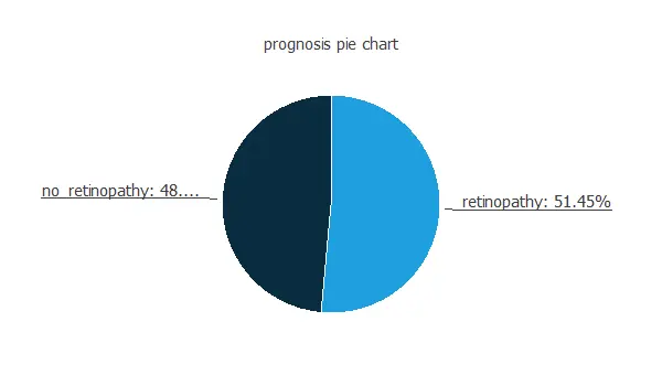
As we can see, the percentage of people who will suffer from diabetic retinopathy in the samples is 48.55%. The ones that will not have it represent 51.45% approximately.
Inputs-targets correlations
Other relevant numbers to remember are the inputs-targets correlations, which indicate what factors influence the disease the most.
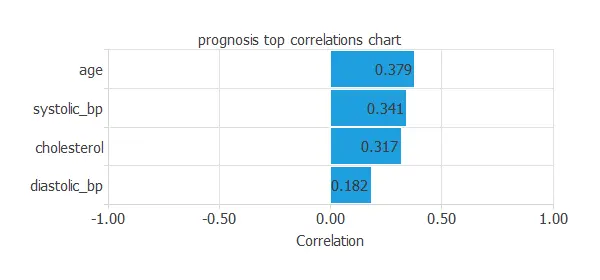
From the picture above, we can gather that all the variables have a similar influence on the target variable, except for the diastolic blood pressure, which is less related.
3. Neural network
The second step is to set a neural network representing the classification function. Classification models usually contain the following layers:
- Scaling layer.
- Perceptron layers.
- Probabilistic layer.
The scaling layer contains the statistics on the inputs calculated from the data file and the method for scaling the input variables. Here, we set the minimum-maximum method.
Next, we use a perceptron layer with a hyperbolic tangent layer. The neural network must have four inputs, one for each input variable and one output for the target variable. As an initial guess, we use three neurons in the hidden layer.
The probabilistic layer only contains the method for interpreting the outputs as probabilities. As the output layer’s activation function is the logistic function, the output can already be understood as a probability of class membership.
The following figure is a graphical representation of this neural network for diabetic retinopathy prognosis.
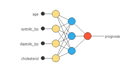
The yellow circles represent scaling neurons, the blue circles represent perceptron neurons, and the red circles represent probabilistic neurons. The number of inputs is 4, and the number of outputs is 1.
4. Training strategy
The fourth step is to set the training strategy, this comprises two terms:
- A loss index.
- An optimization algorithm.
The loss index is the weighted squared error with L1 regularization. This is the default loss index for binary classification models.
The learning problem is finding a neural network that minimizes the loss index. That is a neural network that fits the data set (error term) and does not oscillate (regularization term).
The optimization algorithm that we use is the quasi-Newton method. This is also the standard optimization algorithm for this type of problem.
The following chart shows how errors decrease with each iteration during training. The final training and selection errors are training error = 0.681 WSE and selection error = 0.705 WSE, respectively.
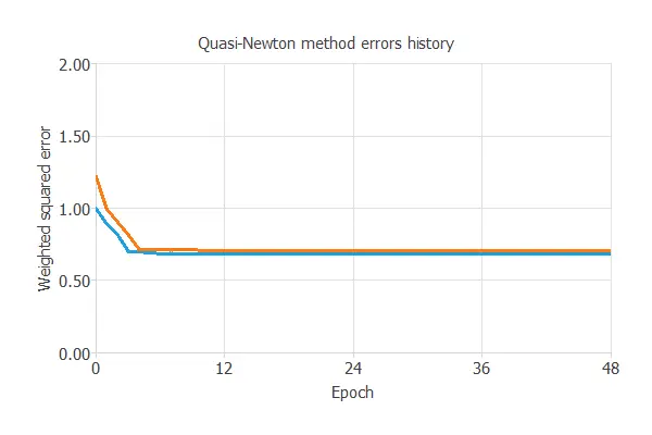
The blue line represents the training error, and the orange is the selection error. The initial value of the training error is 0.950331, and the final value after 48 epochs is 0.673678. The initial value of the selection error is 1.06847, and the absolute value after 48 epochs is 0.682127.
5. Model selection
The objective of model selection is to find the network architecture with the best generalization properties, which minimizes the error on the selected instances of the data set.
More specifically, we want to find a neural network with a selection error of less than 0.705 WSE, the value we have achieved so far.
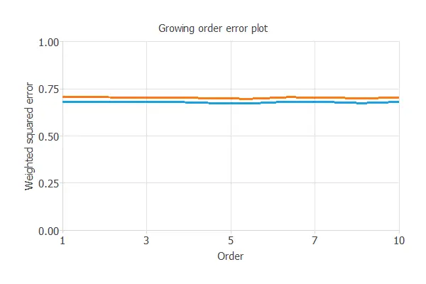
Order selection algorithms train several network architectures with different numbers of neurons or inputs and choose that with the smallest selection error.
The incremental order method starts with a few neurons and increases the complexity at each iteration. The following chart shows the training error (blue) and the selection error (orange) as a function of the number of neurons.
The figure below shows the final architecture for the neural network. We can see that it does not use the diastolic bp input. The results we obtained for the inputs-targets correlations support this.
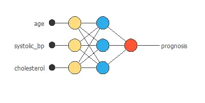
The number of inputs is 3, and the number of outputs is 1. Therefore, the complexity of the number of hidden neurons is 3: 3: 1.
6. Testing analysis
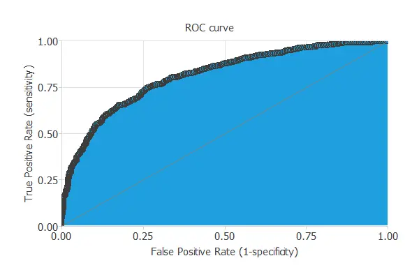
The objective of the testing analysis is to validate the generalization performance of the trained neural network. To validate a classification model, we need to compare the values provided by this model to the observed values. We can use the ROC curve as it is the standard testing method for binary classification projects.
The following table contains the elements of the confusion matrix. This matrix contains the true positives, false positives, false negatives, and true negatives for the variable diagnosis. The total number of testing samples is 1200. The number of correctly classified samples is 893 (74%), and the number of misclassified samples is 307 (25%).
| Predicted positive | Predicted negative | |
|---|---|---|
| Real positive | 464 (38%) | 145 (12%) |
| Real negative | 162 (13%) | 429 (35%) |
The binary classification tests are parameters for measuring the performance of a classification problem with two classes:
- Classification accuracy (ratio of instances correctly classified): 74.33%
- Error rate (ratio of instances misclassified): 25.66%
- Sensitivity (ratio of real positive which are predicted positive): 75.041%
- Specificity (ratio of real negative which are predicted negative): 74.11%
7. Model deployment
Once testing the neural network’s generalization performance, one can save the neural network for future use in the so-called model deployment mode.
We can prognosticate new patients by calculating the neural network outputs. For that, we need to know the input variables for them. An example is the following:
- age: 55
- systolic_bp: 100.89 mmHg
- cholesterol: 140.78 mg/dl
- prognosis: 0.85, so the patient has 85% probability of suffering diabetic retinopathy.
We can also use Response Optimization. The objective of the response optimization algorithm is to exploit the mathematical model to look for optimal operating conditions.
An example is to minimize the probability of suffering diabetic retinopathy while maintaining the age between two values.
The next table resumes the conditions for this problem.
| Variable name | Condition | ||
|---|---|---|---|
| Age | Between | 65 | 95 |
| Systolic bp | None | ||
| Diastolic bp | None | ||
| Cholesterol | None | ||
| Prognosis | Minimize |
The next list shows the optimum values for previous conditions.
- age: 65.
- systolic_bp: 72.23 mmHg.
- diastolic_bp: 93.89 mmHg.
- cholesterol: 84.46 mg/dl.
- prognosis: 23.69%.
The mathematical expression represented by the neural network is written below. It takes age, systolic_bp, and cholesterol to produce the output prognosis. Classification models propagate the information feed-forward through the scaling, perceptron, and probabilistic layers.
scaled_age = age*(1+1)/(103.2789993-(35.16479874))-35.16479874*(1+1)/(103.2789993-35.16479874)-1;
scaled_systolic_bp = systolic_bp*(1+1)/(151.6999969-(69.67539978))-69.67539978*(1+1)/(151.6999969-69.67539978)-1;
scaled_cholesterol = cholesterol*(1+1)/(148.2339935-(69.96749878))-69.96749878*(1+1)/(148.2339935-69.96749878)-1;
perceptron_layer_0_output_0 = sigma[ 0.851161 + (scaled_age*1.62563)+ (scaled_systolic_bp*1.05418)+ (scaled_cholesterol*1.01386) ];
perceptron_layer_0_output_1 = sigma[ 0.688599 + (scaled_age*1.48316)+ (scaled_systolic_bp*1.12786)+ (scaled_cholesterol*0.744651) ];
perceptron_layer_0_output_2 = sigma[ -1.40861 + (scaled_age*-2.32242)+ (scaled_systolic_bp*-1.61186)+ (scaled_cholesterol*-1.35143) ];
probabilistic_layer_combinations_0 = -0.31941 +2.39474*perceptron_layer_0_output_0 +2.16092*perceptron_layer_0_output_1 -3.6845*perceptron_layer_0_output_2
prognosis = 1.0/(1.0 + exp(-probabilistic_layer_combinations_0);
The above expression can be exported anywhere, for instance, to a diagnosis software to be used by doctors.
The file diabetic-retinopathy.py implements the mathematical expression of the neural network in Python. This software can be embedded in any tool to make predictions on new data.
8. Tutorial video
You can watch the step by step tutorial video below to help you complete this Machine Learning example
for free with the easy-to-use machine-learning software Neural Designer.
References
- The data for this problem has been taken from the Coursera repository.