This example assesses the risk of a patient with colorectal cancer of developing liver metastasis. We use mutational data from 492 genes and phenotypic variables using machine learning.
Contents
- Application type.
- Data set.
- Neural network.
- Training strategy.
- Model selection.
- Testing analysis.
- Model deployment.
This example is solved with Neural Designer. You can follow it step by step using the free trial.
1. Application type
The predicted variable can have two values, “yes” if the patient has liver metastasis and “no” otherwise. Therefore, this is a binary classification project.
The goal is to model the probability of metastasis in the liver based on mutational and phenotypic data using artificial intelligence and machine learning.
2. Data set
The liver_metastasis_colon_cancer.csv file contains the data for this example. Target variables can only have two values in a classification model: 0 (false, no) or 1 (true, yes). The number of instances (rows) in the data set is 3537, and the number of variables (columns) is 510.
The number of input variables, or attributes for each sample, is 509. The target variable is 1, distant_metastasis_liver (Yes or No), whether or not the patient has liver metastasis. The following list summarizes the variables information:
- age_at_first_metastasis_diagnostic: age of first metastasis diagnostic.
- age_at_surgical_procedure: age of surgical procedure.
- cancer_type_detailed: cancer type detailed (colon, rectal, colorectal).
- mortality_3_years: whether or not the patient is alive 3 years since their cancer is sequenced.
- fraction_genome_altered: percentage of the genome that has been affected by copy number gains or losses.
- metastasis_count: total number of metastases.
- metastasis_primary_site_count: number of metastases in the primary site.
- microsatellite_instability_score: score regarding the microsatellite instability status.
- microsatellite_instability_type: category for the microsatellite instability assigned based on the msi_score; stable, instable or indeterminate.
- mutation_count: total number of mutated genes from the panel.
- primary_tumor_site: histological localization of the tumor.
- race_category: ethnicity of the patient.
- sex: male or female.
- cancer_subtype: tumor subdivision between microsatellite stable or microsatellite hypermutated.
- tumour_mutational_burden: tumor mutational burden of the total number of non-synonymous somatic mutations identified (those changes in the DNA result in changes in the protein.
- tumor_purity: proportion of cancer cells in the tumor tissue.
- gene_panel: 492 gene panel with the times that a gene is mutated.
To start, we use all instances. Each instance contains the input and target variables of a different patient. The data set is divided into training, validation, and testing subsets. Neural Designer automatically assigns 60% of the instances for training, 20% for selection, and 20% for testing. The user can choose to modify these values to the desired ones.
Also, we can calculate the distributions for all variables. The following figure is a pie chart showing which patients had liver metastasis in the data set.

The image shows that metastatic liver tumors represent 57% of the samples, while 43% represent tumors without liver metastases.
The inputs-targets correlations might indicate to us which factors most influence whether a tumor produces liver metastases or not and, therefore, be more relevant to our analysis.
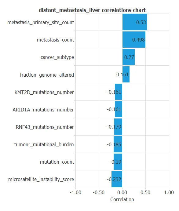
Here, the most correlated variables with malignant tumors are metastasis_primary_site_count, metastasis_count, cancer_subtype, and microsatellite_instability_score.
3. Neural network
The next step is to set up a neural network representing the classification function. For this class of applications, the neural network is composed of:
The scaling layer contains the statistics on the inputs calculated from the data file and the method for scaling the input variables. Here, the minimum-maximum method has been set. Nevertheless, the mean-standard deviation method would produce very similar results. As we use 497 input variables, the scaling layer has 497 inputs.
We won’t use a perceptron layer to stabilize and simplify our model.
The probabilistic layer only contains the method for interpreting the outputs as probabilities. Moreover, as the output layer’s activation function is logistic, that output can already be interpreted as a probability of class membership. The probabilistic layer has 497 inputs. It has one output, representing the probability of a sample being a malignant tumor.
The following figure is a graphical representation of this neural network for liver metastasis diagnosis.
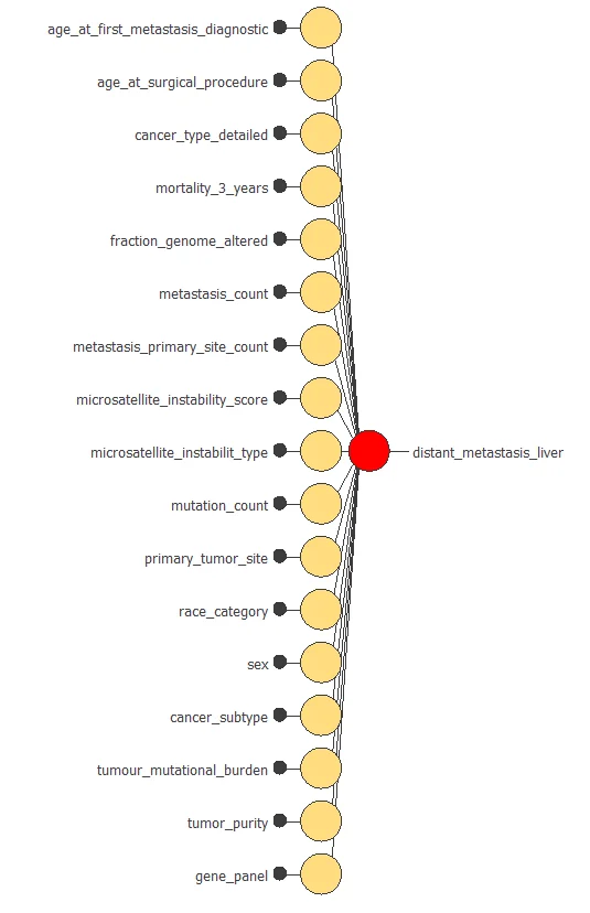
As mentioned above, the network has 497 inputs, from which we obtain a single output value. This value is the probability of liver metastasis for each patient.
4. Training strategy
The fourth step is to set the training strategy, which is composed of two terms:
- A loss index.
- An optimization algorithm.
The loss index is the weighted squared error with L2 regularization, which is the default loss index for binary classification applications.
We can state the learning problem as finding a neural network that minimizes the loss index. That is a neural network that fits the data set (error term) and does not oscillate (regularization term).
The optimization algorithm that we use is the quasi-Newton method, which is also the standard optimization algorithm for this type of problem.
The following chart shows how the error decreases with the iterations during the training process. The final training and selection errors are training error = 0.3969 WSE and selection error = 0.8127 WSE, respectively.
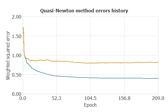
As we can see in the previous image, the curves have converged, although the selection error is greater than the training error, so we could try to continue improving the model to further reduce the errors.
5. Model selection
The objective of model selection is to find the network architecture that minimizes the error, that is, with the best generalization properties for the selected instances of the data set.
Order selection algorithms train several network architectures with different number of neurons and select that with the smallest selection error. We have removed our perceptron layer to stabilize our model, so we cannot use this feature.
However, we will use input selection to select features in the data set that provide the best generalization capabilities.
In the following image, we see that we can reduce the training/selection error using this method.
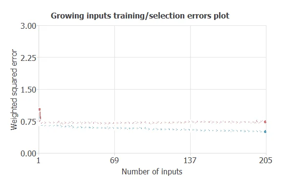
Ultimately, we obtain a training error = 0.6333 WSE and selection error = 0.6264 WSE, respectively. Also, we have reduced the number of inputs to only 18 features. Our network is now like this:
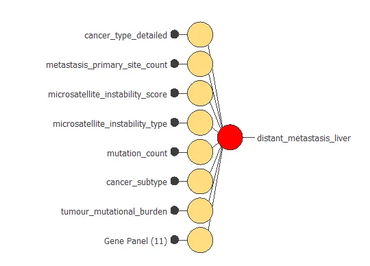
Our final network, has 7 inputs corresponding to phenotypic variables, and 11 Genes from the panels, for a total of 18 input variables. The genes are: KIT, CARD11, RB1, WT1, PLCG2, DNMT1, BRD4, PIK3R1, IRS2, SESN1, NPM1.
6. Testing analysis
The objective of the testing analysis is to validate the performance of the generalization properties of the trained neural network. To validate a classification technique, we need to compare the values provided by this technique to the observed values. We can use the ROC curve as it is the standard testing method for binary classification projects.
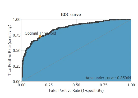
A random classifier has an area under a curve of 0.5, while a perfect classifier has a value of 1. The closer this value is to 1, the better the classifier. In this example, this parameter is AUC = 0.85, which means a great performance.
The following table contains the elements of the confusion matrix. This matrix contains the true positives, false positives, false negatives, and true negatives for the variable diagnosis.
| Predicted negative | Predicted positive | |
|---|---|---|
| Real negative | 344 (48.7%) | 69 (9.8%) |
| Real positive | 86 (12.2%) | 208 (29.4%) |
The binary classification tests are parameters for measuring the performance of a classification problem with two classes:
- Classification accuracy (ratio of instances correctly classified): 78%
- Error rate (ratio of instances misclassified): 21.9%
- Specificity (ratio of real positive which are predicted positive): 70.7%
- Sensitivity (ratio of real negative which are predicted negative): 83.3%
7. Model deployment
Once we have tested the neural network’s generalization performance, we can save it for future use in the so-called model deployment mode.
The mathematical expression represented by the neural network is written below.
scaled_Colon Adenocarcinoma = Colon Adenocarcinoma*(1+1)/(1-(0))-0*(1+1)/(1-0)-1;
scaled_Rectal Adenocarcinoma = Rectal Adenocarcinoma*(1+1)/(1-(0))-0*(1+1)/(1-0)-1;
scaled_Colorectal Adenocarcinoma = Colorectal Adenocarcinoma*(1+1)/(1-(0))-0*(1+1)/(1-0)-1;
scaled_metastasis_primary_site_count = (metastasis_primary_site_count-3.15437007)/2.403779984;
scaled_microsatellite_instability_score = (microsatellite_instability_score-3.579030037)/9.864089966;
scaled_Stable = Stable*(1+1)/(1-(0))-0*(1+1)/(1-0)-1;
scaled_Indeterminate = Indeterminate*(1+1)/(1-(0))-0*(1+1)/(1-0)-1;
scaled_Instable = Instable*(1+1)/(1-(0))-0*(1+1)/(1-0)-1;
scaled_Do not report = Do not report*(1+1)/(1-(0))-0*(1+1)/(1-0)-1;
scaled_mutation_count = (mutation_count-13.76679993)/27.63050079;
scaled_cancer_subtype = cancer_subtype*(1+1)/(1-(0))-0*(1+1)/(1-0)-1;
scaled_tumour_mutational_burden = (tumour_mutational_burden-12.34119987)/24.77930069;
scaled_KIT_mutations_count = (KIT_mutations_count-0.02431439981)/0.1713950038;
scaled_CARD11_mutations_count = (CARD11_mutations_count-0.0667231977)/0.2999680042;
scaled_RB1_mutations_count = (RB1_mutations_count-0.02685889974)/0.1964139938;
scaled_WT1_mutations_count = (WT1_mutations_count-0.01809439994)/0.1435080022;
scaled_PLCG2_mutations_count = (PLCG2_mutations_count-0.04156060144)/0.2185139954;
scaled_DNMT1_mutations_count = (DNMT1_mutations_count-0.03901610151)/0.2357760072;
scaled_BRD4_mutations_count = (BRD4_mutations_count-0.03647160158)/0.2033720016;
scaled_PIK3R1_mutations_count = (PIK3R1_mutations_count-0.05597959831)/0.268456012;
scaled_IRS2_mutations_count = (IRS2_mutations_count-0.04014699906)/0.2343810052;
scaled_SESN1_mutations_count = (SESN1_mutations_count-0.006219959818)/0.08213800192;
scaled_NPM1_mutations_count = NPM1_mutations_count*(1+1)/(1-(0))-0*(1+1)/(1-0)-1;

probabilistic_layer_combinations_0 = 0.0150952 +0.157874*scaled_Colon Adenocarcinoma -0.154215*scaled_Rectal Adenocarcinoma -0.0195006*scaled_Colorectal Adenocarcinoma +1.68684*metastasis_primary_site_count +0.158263*scaled_microsatellite_instability_score -0.066526*scaled_Stable +0.547837*scaled_Indeterminate -0.471286*scaled_Instable -0.0375401*scaled_Do not report -0.181048*scaled_mutation_count +0.611953*scaled_cancer_subtype +0.0808695*scaled_tumour_mutational_burden -0.0273534*scaled_KIT_mutations_count +0.0444354*scaled_CARD11_mutations_count +0.0211164*scaled_RB1_mutations_count +0.0739666*scaled_WT1_mutations_count +0.0429152*scaled_PLCG2_mutations_count +0.00816219*scaled_DNMT1_mutations_count -0.138295*scaled_BRD4_mutations_count +0.0240884*scaled_PIK3R1_mutations_count +0.0625585*scaled_IRS2_mutations_count +0.0364737*scaled_SESN1_mutations_count +0.0926002*scaled_NPM1_mutations_count

distant_metastasis_liver = 1.0/(1.0 + exp(-probabilistic_layer_combinations_0);
The above expression can be exported anywhere, for instance, to a dedicated diagnosis software doctors use. It can even be integrated into a website:
Please note that it is impossible to predict the future with certainty, and a physician must always interpret these predictions to make a diagnosis.
References
- The data for this problem has been taken from the cBioportal Repository MSK-MET (Memorial Sloan Kettering – Metastatic Events and Tropisms) dataset.
