The primary objective is to develop a machine learning model for classifying asteroid orbits.
Contents
1. Application type
This is a classification project since the variable to be predicted is categorical: AMO, APO, ATE.
These orbit types refer to asteroid orbits, allowing the model to categorize orbits according to the aforementioned asteroid orbit classes.
2. Data set
The first step is to prepare the dataset, which serves as the source of information for the classification problem.
For that, we need to configure the following concepts:
- Data source.
- Variables.
- Instances.
Data source
The number of columns is 12, and the number of rows is 1722.
Variables
The variables are:
Orbital Parameters
- a (Semi-major axis): Average distance between the object and the Sun, measured in astronomical units (AU).
- e (Eccentricity): Measure of how elongated the orbit is (0 = circular, closer to 1 = more elliptical).
- i (Inclination): Tilt of the orbit relative to the ecliptic plane (J2000), measured in degrees.
- w (Argument of perihelion): Angle from the ascending node to the orbit’s closest approach to the Sun, measured in degrees.
- Node (Longitude of ascending node): Angle from the reference direction to the ascending node, measured in degrees.
- M (Mean anomaly): Angle describing the position of the object in its orbit at a specific time (epoch), measured in degrees.
Distances & Period
- q (Perihelion distance): Closest distance between the object and the Sun, in AU.
- Q (Aphelion distance): Farthest distance between the object and the Sun, in AU.
- P (Orbital period): Time the object takes to complete one orbit, measured in Julian years.
Physical & Safety Indicators
- H (Absolute V-magnitude): Brightness of the object as observed from a standard distance, related to size.
- MOID (Minimum Orbit Intersection Distance): Closest possible distance between the orbit of the object (NEO) and Earth’s orbit.
Target Variable
Class: Orbital classification (AMO, APO, ATE).
By definition, Atens are Earth-crossing asteroids (a<1.0 AU and Q>0.983 AU).
These different asteroid orbits are shown in the following image:
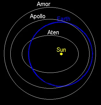
Note that neural networks work with numbers. In this regard, the categorical variable “class” is transformed into three numerical variables as follows:
- AMO: 1 0 0.
- APO: 0 1 0.
- ATE: 0 0 1.
Instances
Variables distributions
We can calculate the distributions of all variables.
The following figure is a pie chart showing the various orbit types.
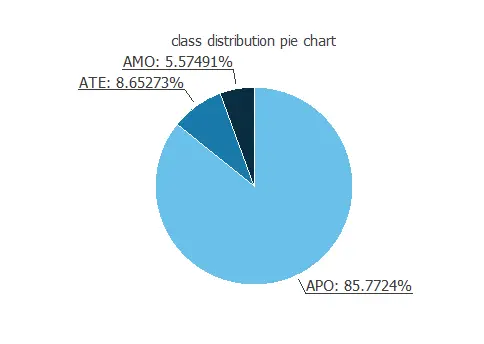
As we can see, most of the samples are APO orbits.
Inputs-targets correlations
Finally, the input-target correlations might indicate to us what factors most influence.
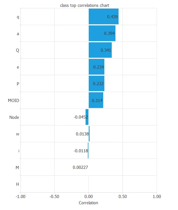
Here, the most correlated variables with the classification are q and Q, the semi-major axis, perihelion distance, and aphelion distance of the orbit.
Additionally, there are a few correlated variables, such as M, mean anomaly, or H, absolute V magnitude.
3. Neural network
The second step is to choose a neural network for classification.
- A scaling layer.
- A hidden dense layer.
- An output dense layer.
Scaling layer
The scaling layer contains the statistics on the inputs calculated from the data file and the method for scaling the input variables.
Hidden dense layer
The hidden dense layer has 11 inputs and 3 neurons.
Output dense layer
The output dense layer allows the outputs to be interpreted as probabilities. All outputs are between 0 and 1, and their sum is 1.
The softmax probabilistic method is used here. The neural network has three outputs since the target variable contains 3 classes (AMO, APO, ATE).
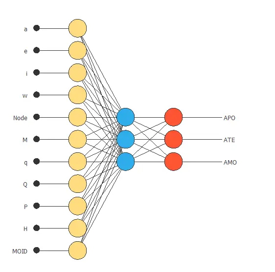
Neural network graph
The following figure is a graphical representation of this classification neural network.
Here, the yellow circles represent scaling neurons, the blue circles represent perceptron neurons, and the red circles represent probabilistic neurons.
4. Training strategy
The fourth step is to set the training strategy, which is composed of:
- Loss index.
- Optimization algorithm.
Loss index
The loss index chosen for this application is the normalized squared error with L2 regularization.
The error term fits the neural network to the training instances of the data set. The regularization term makes the model more stable and improves generalization.
Optimization algorithm
The optimization algorithm searches for the neural network parameters that minimize the loss index. The quasi-Newton method is chosen here.
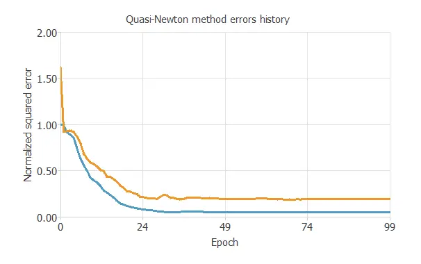
Training
The following chart shows how training and selection errors decrease with the epochs during training.
5. Model selection
The objective of model selection is to find the network architecture with the best generalization properties, which minimizes the error on the selected instances of the data set.
Order selection algorithms train several network architectures with different numbers of neurons and select the one with the smallest selection error.
The incremental order method starts with a few neurons and increases the complexity at each iteration.
6. Testing analysis
The purpose of the testing analysis is to validate the model’s generalization performance.
Here, we compare the neural network outputs to the corresponding targets in the test instances of the dataset.
Confusion matrix
The diagonal cells show the correctly classified cases, and the off-diagonal cells show the misclassified cases.
| Predicted APO | Predicted ATE | Predicted AMO | |
|---|---|---|---|
| Real APO | 283 (84.0%) | 0 (0.0%) | 1 (0.3%) |
| Real ATE | 1 (0.3%) | 30 (8.7%) | 0 (0.0%) |
| Real AMO | 7 (2.0%) | 0 (0.0%) | 16 (4.7%) |
As we can see, the model correctly predicts 335 instances (97.4%), while misclassifying 9 (2.6%).
This indicates that our predictive model achieves high classification accuracy.
7. Model deployment
Neural network outputs
We calculate the neural network outputs from the different variables to classify a given orbit.
For instance:
- a: 1.75 AU.
- e: 0.53.
- i: 13.35 degrees.
- w: 180.46 degrees.
- Node: 172.25 degrees.
- M: 180.73 degrees.
- q: 0.76 AU.
- Q: 2.75 AU.
- P: 2.44 yr.
- H: 19.94.
- MOID: 0.02 AU.
- Probability of APO: 99.9%.
- Probability of ATE: ~0.0%.
- Probability of AMO: ~0.0%.
The neural network would classify the orbit as an Apollo asteroid orbit for this case since it has the highest probability.
Conclusions
We have just built a predictive model to determine the possible asteroid orbit type.
References
- Kaggle. Orbit Classification For Prediction.