
Estimate superconducting critical temperature from composition-derived descriptors
This regression benchmark maps 81 engineered physicochemical descriptors to critical temperature. On 4,252 held-out rows, the final 81–13–1 neural network reaches R² = 0.817 and RMSE = 14.88 K. It supports comparative screening of represented materials; it does not determine whether an arbitrary compound is superconducting.
1. Scientific objective
The objective is to estimate a known superconductor’s critical temperature (Tc) from descriptors derived from its elemental composition. The output can help materials-informatics teams rank represented candidates, compare modelling approaches and prioritize experiments. Because the training set contains known superconductors, the model is a temperature regressor—not a classifier of superconducting behaviour.
Candidate ranking
Compare predicted Tc values before allocating higher-cost synthesis and characterization work.
Model benchmarking
Provide a reproducible neural baseline for composition-derived materials descriptors.
Experimental planning
Use predictions with domain checks to support—not replace—physics-informed laboratory decisions.
2. Data and provenance
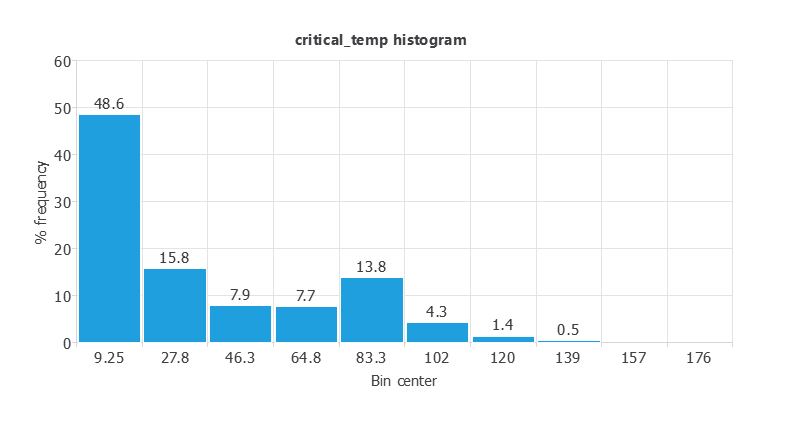
The UCI Superconductivity data set contains 21,263 records with no missing values. The target is critical_temp in kelvin. A reproducible 60/20/20 row split assigns 12,759 records to training, 4,252 to model selection and 4,252 to testing.
Why there are two CSV files
| File | Role | Contents | Use |
|---|---|---|---|
superconductor.csv | Primary modelling data | 81 numeric descriptors plus critical_temp | Train, validate and run the published model |
chemical_compounds.csv | Auxiliary composition table | 86 elemental stoichiometry columns, critical_temp and formula | Identify materials and connect model rows with chemical formulas |
The files contain the same 21,263 row-aligned target observations but serve different purposes. Keeping both avoids pretending that the exported network accepts a chemical formula directly.
Descriptor design
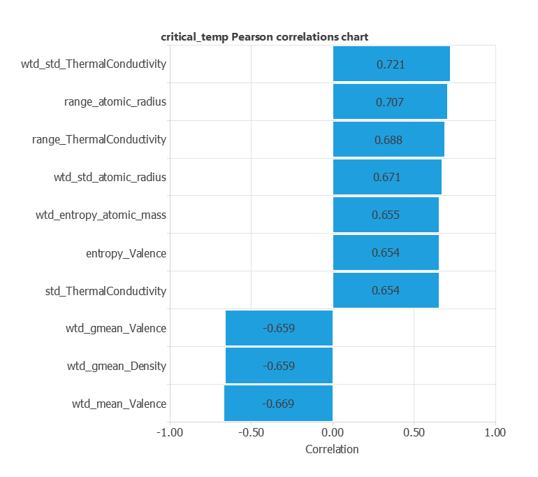
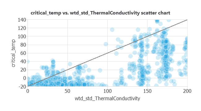
The 81 inputs comprise number_of_elements plus ten statistics for each of eight elemental properties: atomic mass, first ionization energy, atomic radius, density, electron affinity, heat of fusion, thermal conductivity and valence. The statistics are mean, weighted mean, geometric mean, weighted geometric mean, entropy, weighted entropy, range, weighted range, standard deviation and weighted standard deviation.
| Subset | Rows | Purpose |
|---|---|---|
| Training | 12,759 | Estimate network parameters |
| Selection | 4,252 | Select hidden-layer size |
| Testing | 4,252 | Final held-out evaluation |
3. Model
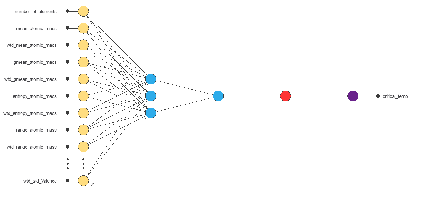
The modelling process starts with an 81–3–1 baseline. All 81 inputs use mean-and-standard-deviation scaling; a dense hidden layer with three tanh neurons learns nonlinear descriptor interactions, and an identity output neuron returns Tc before output unscaling. This initial network contains 250 trainable parameters and provides the reference architecture for training and neuron selection.
4. Training strategy
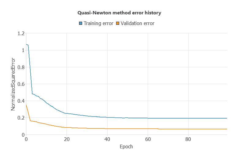
The network minimizes normalized squared error with L2 regularization of 0.01 using the Quasi-Newton method. The initial three-neuron network finishes with training error 0.192 and selection error 0.0668 after 99 iterations.
5. Model selection and baseline
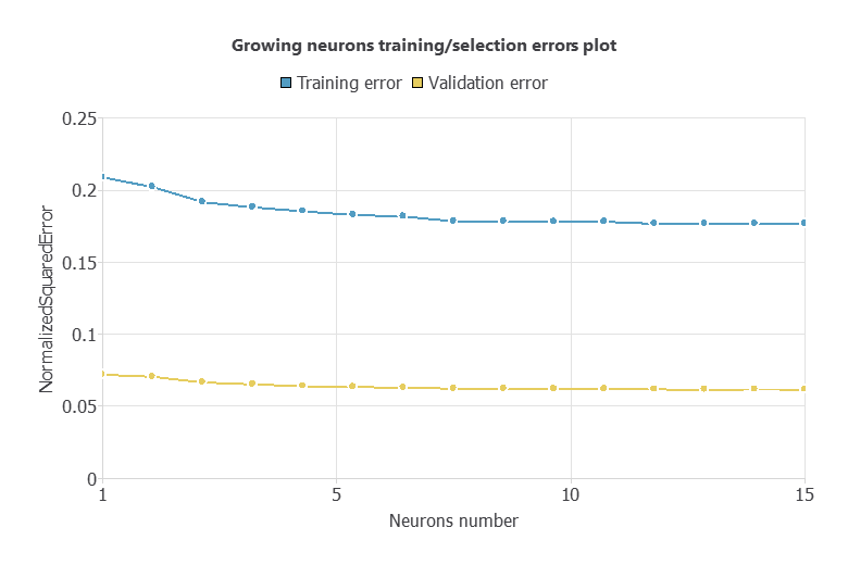
Neuron selection evaluates one to 15 hidden neurons while keeping the data partition and training strategy fixed. The minimum selection error is 0.0616 at 13 neurons, approximately 7.4% below the three-neuron result; the final model therefore uses 13 hidden neurons.
Selected architecture
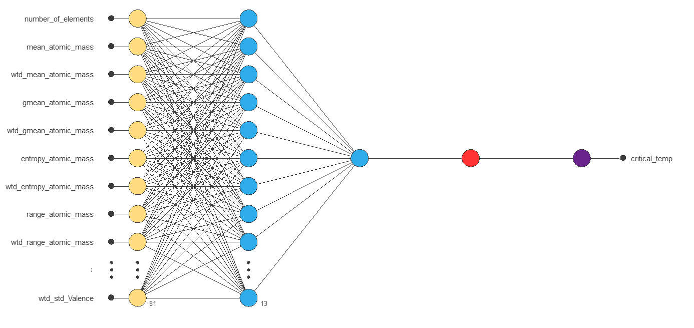
After neuron selection, the hidden layer is expanded from three to 13 tanh neurons. The resulting 81–13–1 network contains 1,080 trainable parameters and is the model used for testing, deployment and the downloadable Python export.
| Reference | Testing RMSE | Interpretation |
|---|---|---|
| Training-mean baseline | 34.81 K | Null predictor using one constant value |
| Final neural network | 14.88 K | 57% lower RMSE than the null baseline |
6. Scientific validation
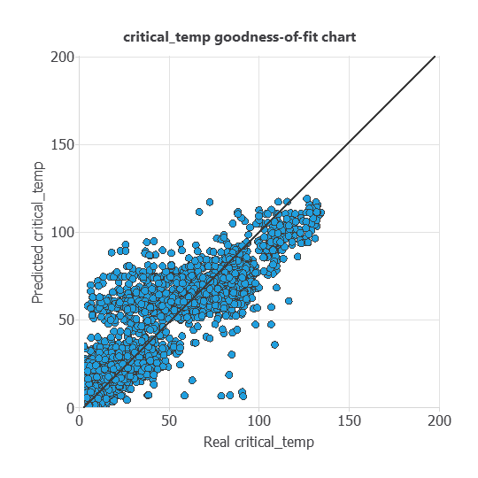
Final metrics are calculated only on the 4,252 testing rows. R² measures explained test variance; RMSE emphasizes large misses; MAE gives a more direct typical error; signed bias checks systematic over- or underprediction.
| Metric | Testing result | Reading |
|---|---|---|
| R² | 0.817 | 81.7% of testing variance explained |
| RMSE | 14.88 K | Penalizes larger temperature errors |
| MAE | 10.32 K | Mean absolute testing error |
| Mean signed error | −0.28 K | Small overall bias can hide regional bias |
| Prediction-vs-observation slope | 0.801 | Compression toward the middle of the range |
Performance by observed temperature
| Observed Tc band | Testing rows | MAE | Mean signed error |
|---|---|---|---|
| 0–20 K | 2,130 | 6.57 K | +3.37 K |
| 20–77 K | 1,305 | 12.24 K | +3.76 K |
| 77–120 K | 768 | 16.69 K | −15.84 K |
| 120–186 K | 49 | 22.61 K | −22.61 K |
7. Inference and reproducibility
A credible deployment begins with a formula or composition record, generates the same 81 descriptors, validates names, order and applicability ranges, calculates Tc and routes the estimate—together with model version and warnings—to scientific review.
Three representative inference cases
Neural Designer’s output-data task was run on three descriptor vectors taken from the primary table. Their formulas were recovered from the row-aligned auxiliary composition table, and the same inputs were then evaluated with the exported Python model.
| Material | Formula | Observed Tc | Predicted Tc | Signed error |
|---|---|---|---|---|
| Mercury | Hg | 4.16 K | 4.83 K | +0.67 K |
| Magnesium diboride | MgB2 | 39.00 K | 31.22 K | −7.78 K |
| YBCO | YBa2Cu3O7 | 92.00 K | 73.77 K | −18.23 K |
These are transparent calculation examples, not an additional validation set. They make the operational pattern visible: the low-Tc case is close, while the high-Tc YBCO case is substantially underestimated. Multiple experimental records can share the same composition-derived vector but report different Tc values, because conditions absent from the descriptors can matter.
Reproduce the calculation
The Python package contains the exact final export, the ordered 81-input schema, the three deployment rows and their calculated outputs. The compact Neural Designer project excludes obsolete embedded data from an earlier configuration.
import pandas as pd
from model import NeuralNetwork

cases = pd.read_csv("deployment_cases.csv", sep=";")
model = NeuralNetwork()
assert list(cases.columns) == model.input_names
predicted_tc_K = model.calculate_batch_output(
    cases.to_numpy(dtype=float)
)[:, 0]8. Validity, uncertainty and limitations
- Applicability is restricted. The source contains known superconductors; the model neither discovers superconductivity nor establishes that an arbitrary compound has a nonzero Tc.
- Composition is incomplete physics. Crystal structure, pressure, synthesis route, stoichiometric uncertainty and measurement conditions are absent.
- The row-random split is optimistic. About 33.4% of testing rows have an exact engineered descriptor vector in training. On unseen descriptor vectors, R² falls to 0.801 and RMSE rises to 15.32 K.
- Repeated formulas are not independent experiments. Formula-level or material-family grouping is preferable when estimating transfer to new chemistries.
- High-Tc estimates are systematically compressed. The 77–120 K and 120–186 K bands show mean underprediction of 15.84 K and 22.61 K respectively.
- Raw output requires a physical guard. The stored test predictions include 202 negative values; these must be flagged as non-physical and investigated rather than silently accepted.
- No external material-family validation is shown. Before laboratory use, compare against grouped cross-validation, uncertainty estimates and truly external compounds.
References
- UCI Machine Learning Repository: Superconductivity Data (DOI: 10.24432/C53P47; CC BY 4.0).
- K. Hamidieh, A data-driven statistical model for predicting the critical temperature of a superconductor, Computational Materials Science 154 (2018), 346–354.
- National Institute for Materials Science: SuperCon data resources.